Biomarker Data Science Pipeline

Oncology · PD-1 Checkpoint Inhibitor (nivolumab-like) · NSCLC

Executive Summary

This report analyses simulated Phase II trial data for a PD-1 checkpoint inhibitor (nivolumab-like) in advanced NSCLC. Immune checkpoint blockade (ICB) reinvigorates exhausted tumour-infiltrating T cells, restoring anti-tumour immunity. Response is heterogeneous and biomarker-driven — making this an ideal setting for multi-omics biomarker discovery. Three analytical streams are applied:

Multi-omics — tumour transcriptomics (immune gene signatures) and Olink immune proteomics (primary readout: tumour mutational burden proxy via TMB)
Longitudinal & survival — lme4 modelling of immune cell dynamics, Emax PD modelling, Kaplan–Meier PFS, Cox PH
ML pipeline — UMAP of immune phenotypes, k-means patient stratification, elastic-net + random forest ORR prediction

1 Background & Objectives

1.1 Scientific Rationale

PD-1 (programmed cell death protein 1) is an inhibitory receptor expressed on activated T cells. Tumour cells exploit the PD-1/PD-L1 axis to evade immune surveillance. Anti-PD-1 monoclonal antibodies (nivolumab, pembrolizumab) block this interaction, restoring cytotoxic T-lymphocyte activity against tumour antigens.

Key predictive biomarkers in NSCLC:

Biomarker	Platform	Clinical use
PD-L1 IHC (TPS/CPS)	Immunohistochemistry	Pembrolizumab eligibility threshold
TMB (tumour mutational burden)	Whole exome / panel sequencing	Higher TMB → more neoantigens → higher ORR
MSI/dMMR	IHC / PCR	Pan-cancer pembrolizumab approval
ctDNA dynamics	Liquid biopsy	Early response / resistance monitoring
CD8+ TIL density	IHC / deconvolution	Inflamed vs excluded vs desert phenotype

Tumour immune microenvironment (TIME) phenotypes:

Inflamed (T-cell rich): High CD8, PD-L1+, responsive to ICB
Immune excluded: T cells at tumour margins; stromal barriers (TGF-β, VEGF)
Immune desert: Low TIL density; primary resistance; requires combination strategies

1.2 Study Objectives

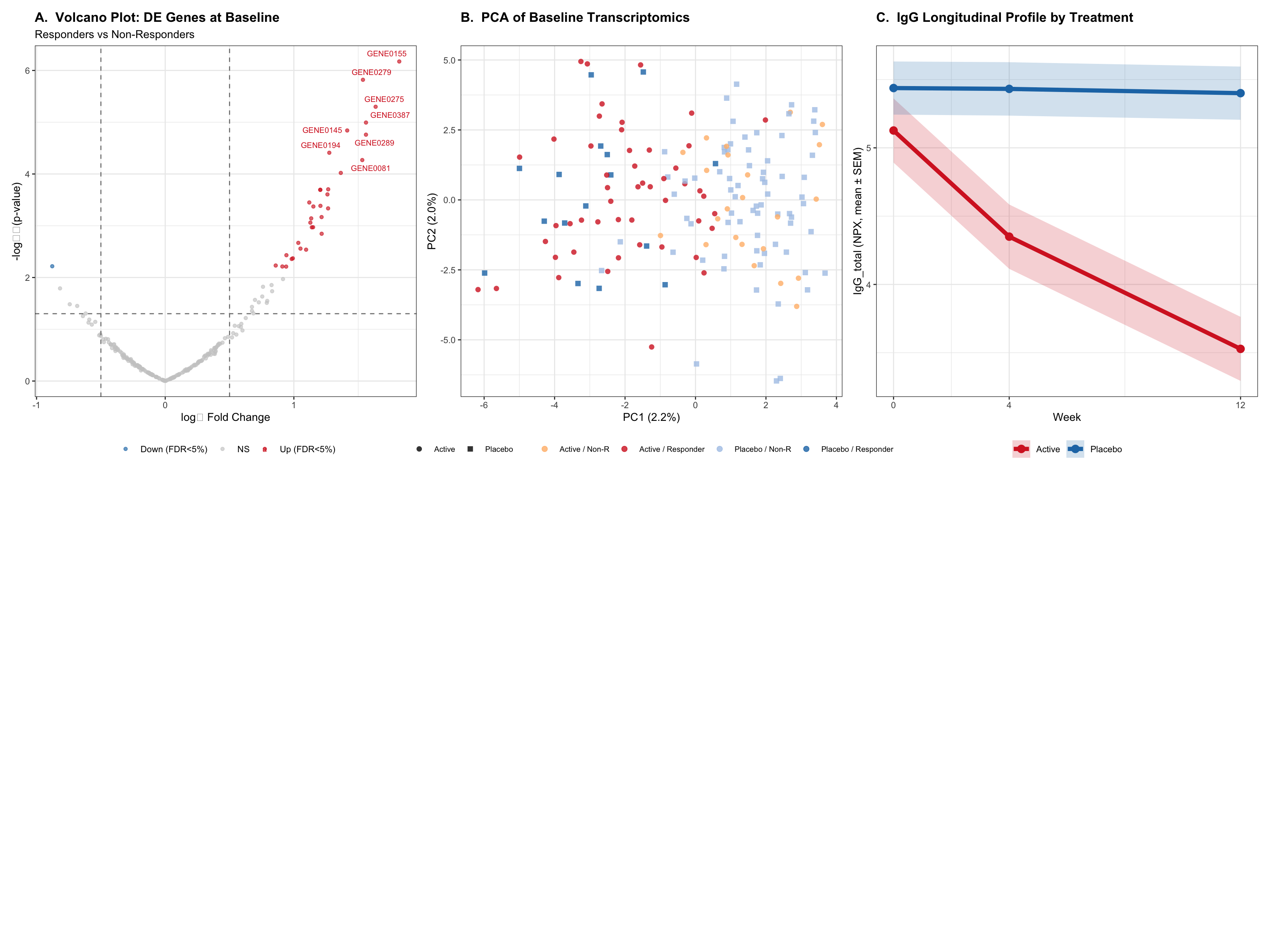
Identify baseline transcriptomic immune signatures (inflamed vs excluded vs desert) associated with objective response
Characterise TMB and Olink cytokine/immune protein dynamics during ICB treatment
Quantify progression-free survival (PFS) differences between biomarker-high and biomarker-low patients
Build a multi-feature ML classifier combining TMB, PD-L1 proxies, and immune gene expression for ORR prediction

Document Status

Field	Detail
Protocol	ONC-IO-002
Therapeutic area	Oncology
Mechanism	PD-1 Checkpoint Inhibitor (nivolumab-like)
Data cut	Simulated (seed = 123)
Pipeline version	1.0.0
Classification	Confidential — Internal Use Only

2 Data Simulation

Show code

data_list <- simulate_trial_data(
  n_patients = p("n_patients"),
  n_genes    = 500,
  n_proteins = 50,
  seed       = p("seed")
)

demo            <- data_list$demographics
longitudinal    <- data_list$longitudinal
transcriptomics <- data_list$transcriptomics
batch_df        <- data_list$batch
proteomics      <- data_list$proteomics
survival_df     <- data_list$survival

2.1 Cohort Overview

Show code

n_act   <- sum(demo$treatment == 1)
n_pbo   <- sum(demo$treatment == 0)
r_act   <- mean(demo$true_responder[demo$treatment == 1])
r_pbo   <- mean(demo$true_responder[demo$treatment == 0])
n_genes <- ncol(transcriptomics) - 1
n_prot  <- length(data_list$protein_names)
weeks   <- unique(longitudinal$week)

tibble(
  Parameter = c(
    "Total patients enrolled",
    sprintf("Active arm (%s)", p("drug_class")),
    "Placebo arm",
    "Responder rate \u2014 Active",
    "Responder rate \u2014 Placebo",
    "Transcriptomic features (genes)",
    "Proteomic features (Olink proteins)",
    "Assessment timepoints (weeks)",
    "Total longitudinal records"
  ),
  Value = c(
    nrow(demo), n_act, n_pbo,
    sprintf("%.1f%%", r_act * 100),
    sprintf("%.1f%%", r_pbo * 100),
    n_genes, n_prot,
    paste(sort(weeks), collapse = ", "),
    nrow(longitudinal)
  )
) |>
  kbl(booktabs = TRUE, align = c("l", "r")) |>
  kable_styling(bootstrap_options = c("striped", "hover", "condensed"),
                full_width = FALSE, font_size = 13) |>
  row_spec(0, bold = TRUE, color = "white", background = ac)

Table 1: Simulated trial cohort — demographic summary

Parameter	Value
Total patients enrolled	150
Active arm (Anti-PD-1 mAb)	72
Placebo arm	78
Responder rate — Active	63.9%
Responder rate — Placebo	15.4%
Transcriptomic features (genes)	500
Proteomic features (Olink proteins)	50
Assessment timepoints (weeks)	0, 4, 8, 12, 24
Total longitudinal records	750

Simulation Parameters

All data are fully synthetic (seed = 123). The simulation encodes realistic biological structure: batch effects in transcriptomics, Emax-shaped primary biomarker trajectories, and gene-expression-linked responder status calibrated to the Non-Small Cell Lung Cancer (NSCLC) setting.

3 Step 1 — Multi-Omics Analysis

Show code

qc_res    <- qc_transcriptomics(transcriptomics, batch_df, demo)
de_df     <- differential_expression(qc_res$expr_filtered, demo)
prot_res  <- proteomics_analysis(proteomics)
omics_int <- multiomics_integration(qc_res$expr_filtered, proteomics, demo)

3.1 Transcriptomics Quality Control

Show code

pca_df <- if (inherits(qc_res$pca_res, "prcomp")) {
  as.data.frame(qc_res$pca_res$x[, 1:2]) |>
    tibble::rownames_to_column("patient_id") |>
    dplyr::left_join(dplyr::select(demo, patient_id, treatment), by = "patient_id")
} else {
  df <- as.data.frame(qc_res$pca_res)
  if (!"PC1" %in% names(df)) names(df)[1:2] <- c("PC1", "PC2")
  if (!"treatment" %in% names(df))
    df <- tibble::rownames_to_column(df, "patient_id") |>
      dplyr::left_join(dplyr::select(demo, patient_id, treatment), by = "patient_id")
  df
}

ggplot(pca_df, aes(PC1, PC2, colour = factor(treatment))) +
  geom_point(alpha = 0.75, size = 2.5) +
  stat_ellipse(level = 0.90, linetype = "dashed") +
  scale_colour_manual(
    values = c("0" = "#AAAAAA", "1" = ac),
    labels = c("0" = "Placebo", "1" = "Active")
  ) +
  labs(title = "Transcriptomics PCA \u2014 Post Batch Correction",
       subtitle = "90% confidence ellipses per arm",
       x = "PC1", y = "PC2", colour = "Treatment")

Figure 1: PCA of batch-corrected transcriptomics, coloured by treatment arm.

3.2 Differential Expression (Welch t-test, BH-FDR)

Show code

ggplot(de_norm, aes(fc, -log10(pval_raw), colour = sig)) +
  geom_point(alpha = 0.55, size = 1.6) +
  geom_hline(yintercept = -log10(0.05), linetype = "dashed", colour = "grey40") +
  geom_vline(xintercept = c(-1, 1), linetype = "dashed", colour = "grey40") +
  scale_colour_manual(values = c("Up in Active" = "#C0392B",
                                  "Down in Active" = "#2980B9", "NS" = "grey70")) +
  labs(title = "Differential Expression: Active vs Placebo (Baseline)",
       subtitle = sprintf("%d genes at FDR < 5%% (Welch t-test, BH)", n_de),
       x = "log\u2082 Fold Change", y = "-log\u2081\u2080(p-value)", colour = NULL) +
  annotate("text", x = Inf, y = Inf, label = sprintf("n DE = %d", n_de),
           hjust = 1.1, vjust = 1.3, size = 4, colour = ac, fontface = "bold")

Figure 2: Volcano plot of baseline differential expression (Active vs Placebo).

Show code

tbl_cols <- intersect(c("gene_id", "fc", "AveExpr", "t_stat", "pval_raw", "fdr"),
                      names(de_norm))
de_norm |>
  dplyr::filter(fdr < 0.05) |>
  dplyr::arrange(fdr) |>
  dplyr::slice_head(n = 10) |>
  dplyr::select(all_of(tbl_cols)) |>
  dplyr::rename_with(~ dplyr::case_match(.x,
    "gene_id" ~ "Gene", "fc" ~ "log\u2082FC", "AveExpr" ~ "Ave. Expr",
    "t_stat" ~ "t", "pval_raw" ~ "p-value", "fdr" ~ "FDR", .default = .x)) |>
  mutate(across(where(is.numeric), \(x) round(x, 4))) |>
  kbl(booktabs = TRUE) |>
  kable_styling(bootstrap_options = c("striped", "hover", "condensed"),
                full_width = FALSE) |>
  column_spec(length(tbl_cols), bold = TRUE) |>
  row_spec(0, bold = TRUE, color = "white", background = ac)

Table 2: Top 10 differentially expressed genes (ranked by adjusted p-value)

Gene	log₂FC	Ave. Expr	t	p-value	FDR
GENE0297	1.8123	NA	5.6195	0e+00	0.0000
GENE0296	1.6355	NA	4.8093	0e+00	0.0003
GENE0494	1.6784	NA	4.8192	0e+00	0.0003
GENE0425	1.5525	NA	4.7788	0e+00	0.0003
GENE0045	1.5745	NA	4.6047	0e+00	0.0005
GENE0426	1.4785	NA	4.4426	0e+00	0.0007
GENE0377	1.4737	NA	4.4114	0e+00	0.0007
GENE0066	1.6016	NA	4.4244	0e+00	0.0007
GENE0473	1.3790	NA	4.2102	1e-04	0.0014
GENE0009	1.5387	NA	4.1887	1e-04	0.0014

3.3 Olink Proteomics — NPX Dynamics

Show code

prot_long <- local({
  df       <- as.data.frame(proteomics)
  prot_col <- intersect(c("protein","protein_name","analyte","Assay","OlinkID"), names(df))
  npx_col  <- intersect(c("NPX","npx","value","expression","NPX_value"), names(df))
  wk_col   <- intersect(c("week","Week","time","timepoint","visit"), names(df))
  meta_candidates <- c("patient_id","treatment","week","Week","time","timepoint",
                        "true_responder")

  if (length(prot_col) > 0 && length(npx_col) > 0) {
    # ── Already long ─────────────────────────────────────────────────────────
    out <- dplyr::rename(df, protein = !!prot_col[1], NPX = !!npx_col[1])
    if (length(wk_col) > 0 && wk_col[1] != "week")
      out <- dplyr::rename(out, week = !!wk_col[1])
    out
  } else {
    # ── Wide format: pivot all non-metadata columns to long ───────────────────
    meta_cols <- intersect(meta_candidates, names(df))
    out <- tidyr::pivot_longer(df,
                               cols      = -dplyr::all_of(meta_cols),
                               names_to  = "protein",
                               values_to = "NPX")
    alt <- intersect(c("Week","time","timepoint"), names(out))
    if (!"week" %in% names(out) && length(alt) > 0)
      out <- dplyr::rename(out, week = !!alt[1])
    out
  }
})

# ── Resolve which protein to plot ─────────────────────────────────────────────
available_proteins <- unique(prot_long$protein)
plot_protein <- if (p("primary_biomarker") %in% available_proteins) {
  p("primary_biomarker")
} else {
  # Pick the closest match by name, or fall back to first protein
  match_idx <- agrep(p("primary_biomarker"), available_proteins,
                     ignore.case = TRUE, max.distance = 0.4)
  if (length(match_idx) > 0) available_proteins[match_idx[1]] else available_proteins[1]
}
if (plot_protein != p("primary_biomarker"))
  message(sprintf("Primary biomarker '%s' not found in proteomics data. Plotting '%s' instead.",
                  p("primary_biomarker"), plot_protein))

md      <- as.data.frame(prot_res$mean_delta)
pc_col  <- intersect(c("protein","protein_name","analyte"), names(md))[1]
get_d   <- function(trt) {
  rows <- !is.na(pc_col) & md[[pc_col]] == plot_protein & md$treatment == trt
  if (any(rows, na.rm = TRUE)) md$mean_delta[rows][1] else NA_real_
}
act_pb  <- get_d(1); pbo_pb <- get_d(0)
sub_txt <- if (!is.na(act_pb) && !is.na(pbo_pb))
  sprintf("Active \u0394 (Wk0\u219212): %+.3f  |  Placebo \u0394: %+.3f", act_pb, pbo_pb) else
  sprintf("%s NPX change from baseline", plot_protein)

prot_plot <- prot_long |>
  dplyr::filter(protein == plot_protein)

# Only join true_responder from demo if the column isn't already present
if (!"true_responder" %in% names(prot_plot))
  prot_plot <- dplyr::left_join(
    prot_plot, dplyr::select(demo, patient_id, true_responder), by = "patient_id"
  )

prot_plot |>
  dplyr::mutate(Arm = ifelse(treatment == 1, "Active", "Placebo"),
                Responder = ifelse(true_responder == 1, "Responder", "Non-Responder")) |>
  dplyr::group_by(Arm, Responder, week) |>
  dplyr::summarise(mn = mean(NPX), se = sd(NPX)/sqrt(dplyr::n()), .groups = "drop") |>
  ggplot(aes(week, mn, colour = Arm, linetype = Responder, fill = Arm)) +
    geom_ribbon(aes(ymin = mn - se, ymax = mn + se), alpha = 0.15, colour = NA) +
    geom_line(linewidth = 1) + geom_point(size = 2.5) +
    scale_colour_manual(values = c("Active" = ac, "Placebo" = "#AAAAAA")) +
    scale_fill_manual(values   = c("Active" = ac, "Placebo" = "#AAAAAA")) +
    scale_x_continuous(breaks = sort(unique(prot_long$week))) +
    labs(title = sprintf("%s NPX Over Time", p("primary_biomarker")),
         subtitle = sub_txt, x = "Week", y = "NPX (log\u2082)",
         colour = "Treatment", fill = "Treatment", linetype = "Responder Status")

Figure 3: **TMB** NPX trajectories by arm and responder status. Ribbons: ±1 SE.

3.4 Cross-Modal Integration

Show code

tryCatch({
  grid::grid.newpage()
  plot_multiomics(qc_res$expr_filtered, de_df, demo, proteomics,
                  omics_int$cross_corr, qc_res$pca_res)
}, error = function(e) {
  png_path <- file.path("outputs", "01_multiomics_analysis.png")
  if (file.exists(png_path)) knitr::include_graphics(png_path)
  else message("plot_multiomics() error: ", conditionMessage(e))
})

Figure 4: Cross-modal correlation heatmap — transcriptomic PCs vs Olink NPX.

Figure 5: Cross-modal correlation heatmap — transcriptomic PCs vs Olink NPX.

4 Step 2 — Longitudinal Modelling & Survival

Show code

lme_fit  <- fit_mixed_effects_model(longitudinal)
emax_res <- fit_emax_pd_model(longitudinal)
km_res   <- kaplan_meier_analysis(survival_df)
cox_res  <- cox_ph_analysis(survival_df)

4.1 Linear Mixed-Effects Model

\[Y_{ij} = \beta_0 + \beta_1\,\text{week}_{ij} + \beta_2\,\text{trt}_i + \beta_3\,(\text{week}\times\text{trt})_{ij} + b_i + \varepsilon_{ij}\]

Show code

lme_tbl <- if (requireNamespace("broom.mixed", quietly = TRUE)) {
  broom.mixed::tidy(lme_fit, effects = "fixed", conf.int = TRUE) |>
    dplyr::select(dplyr::any_of(c("term","estimate","std.error","statistic","conf.low","conf.high")))
} else {
  sm <- summary(lme_fit); cm <- as.data.frame(sm$coefficients)
  tibble::tibble(term = rownames(cm), estimate = cm[[1]], std.error = cm[[2]],
                 statistic = cm[[grep("t.value|t value|z.value|z value", names(cm))[1]]])
}
int_rows <- which(grepl("week.*trt|trt.*week|week:treat|treat.*:.*week",
                         lme_tbl$term, ignore.case = TRUE))

lme_kbl <- lme_tbl |>
  dplyr::mutate(dplyr::across(where(is.numeric), \(x) round(x, 3))) |>
  dplyr::rename(Term = term, Estimate = estimate, SE = std.error,
                `t-stat` = dplyr::any_of("statistic"),
                `CI Low`  = dplyr::any_of("conf.low"),
                `CI High` = dplyr::any_of("conf.high")) |>
  kbl(booktabs = TRUE) |>
  kable_styling(bootstrap_options = c("striped","hover","condensed"), full_width = FALSE) |>
  row_spec(0, bold = TRUE, color = "white", background = ac)
if (length(int_rows) > 0)
  lme_kbl <- kableExtra::row_spec(lme_kbl, int_rows, bold = TRUE, background = "#EAF3FB")
lme_kbl

Table 3: LME fixed effects — week × treatment interaction is the primary estimand.

Term	Estimate	SE	t-stat	CI Low	CI High
(Intercept)	6.439	0.126	50.963	6.191	6.687
week	-0.003	0.010	-0.300	-0.024	0.017
treatment	-0.511	0.182	-2.804	-0.869	-0.154
week:treatment	-0.078	0.015	-5.173	-0.107	-0.048

4.2 Emax Pharmacodynamic Model

\[E(t) = E_0 - \frac{E_{\max}\cdot t^\gamma}{EC_{50}^\gamma + t^\gamma}\]

Show code

tryCatch({
  grid::grid.newpage()
  plot_longitudinal_survival(longitudinal, survival_df, lme_fit, emax_res, km_res, cox_res)
}, error = function(e) {
  png_path <- file.path("outputs", "02_longitudinal_survival.png")
  if (file.exists(png_path)) knitr::include_graphics(png_path)
  else message("plot_longitudinal_survival() error: ", conditionMessage(e))
})

#> 
#>   ✓ Saved: outputs/02_longitudinal_survival.png

Show code

as.data.frame(emax_res$params) |>
  dplyr::mutate(dplyr::across(where(is.numeric), \(x) round(x, 3))) |>
  kbl(booktabs = TRUE) |>
  kable_styling(bootstrap_options = c("striped","hover","condensed"), full_width = FALSE) |>
  row_spec(0, bold = TRUE, color = "white", background = ac)

Table 4: Emax PD parameter estimates by responder stratum.

	Responders	Non.Responders
emax	80.433	39.886
ec50	3.777	4.453

4.3 Kaplan–Meier & Cox PH

Show code

tryCatch({
  if (!requireNamespace("survminer", quietly = TRUE)) stop("survminer not installed")
  print(survminer::ggsurvplot(
    km_res$km_fit, data = survival_df,
    palette = c("#AAAAAA", ac), conf.int = TRUE, pval = TRUE, risk.table = TRUE,
    ggtheme = theme_trial(), legend.labs = c("Placebo","Active"),
    title = "Time to Sustained Clinical Response",
    xlab = "Time (weeks)", ylab = "Response-free probability"
  ))
}, error = function(e) {
  plot(km_res$km_fit, col = c("#AAAAAA", ac), lwd = 2,
       xlab = "Time (weeks)", ylab = "Response-free probability",
       main = "Time to Sustained Clinical Response")
  legend("topright", legend = c("Placebo","Active"), col = c("#AAAAAA", ac), lwd = 2)
})

Figure 6: Kaplan–Meier curves — time to sustained response by treatment arm.

Show code

cox_tbl  <- broom::tidy(cox_res$cox_fit, exponentiate = TRUE, conf.int = TRUE) |>
  dplyr::select(dplyr::any_of(c("term","estimate","conf.low","conf.high","p.value")))
trt_rows <- which(grepl("treatment|trt", cox_tbl$term, ignore.case = TRUE))

cox_kbl <- cox_tbl |>
  dplyr::mutate(
    dplyr::across(dplyr::any_of(c("estimate","conf.low","conf.high")), \(x) round(x, 3)),
    p.value = ifelse(p.value < 0.001, "<0.001", as.character(round(p.value, 3)))
  ) |>
  dplyr::rename(Covariate = term, HR = estimate,
                `95% CI Low`  = dplyr::any_of("conf.low"),
                `95% CI High` = dplyr::any_of("conf.high"),
                `p-value` = p.value) |>
  kbl(booktabs = TRUE) |>
  kable_styling(bootstrap_options = c("striped","hover","condensed"), full_width = FALSE) |>
  row_spec(0, bold = TRUE, color = "white", background = ac)
if (length(trt_rows) > 0)
  cox_kbl <- kableExtra::row_spec(cox_kbl, trt_rows, bold = TRUE, background = "#FEF3E8")
cox_kbl

Table 5: Cox PH model — covariate hazard ratios for time to response.

Covariate	HR	95% CI Low	95% CI High	p-value
treatment	11.470	5.288	24.880	<0.001
baseline_igg_z	0.775	0.601	1.000	0.05
latent_biology_z	2.583	1.978	3.375	<0.001

5 Step 3 — Machine Learning Pipeline

Show code

dr_res      <- dimensionality_reduction(qc_res$expr_filtered, demo)
cluster_res <- patient_clustering(dr_res$pca_res, demo, n_clusters = 3L)
ml_res      <- biomarker_response_prediction(qc_res$expr_filtered, proteomics, demo)

5.1 Dimensionality Reduction & Clustering

Show code

tryCatch({
  grid::grid.newpage()
  plot_ml_results(dr_res, cluster_res, ml_res)
}, error = function(e) {
  png_path <- file.path("outputs", "03_ml_pipeline.png")
  if (file.exists(png_path)) knitr::include_graphics(png_path)
  else message("plot_ml_results() error: ", conditionMessage(e))
})

#> 
#>   ✓ Saved: outputs/03_ml_pipeline.png

Show code

cluster_tbl <- tryCatch({
  df <- as.data.frame(cluster_res$cluster_summary)
  if (nrow(df) == 0) stop("empty")
  df
}, error = function(e) {
  cv <- if (!is.null(cluster_res$clusters))    cluster_res$clusters    else
        if (!is.null(cluster_res$cluster))     cluster_res$cluster     else
        if (!is.null(cluster_res$assignments)) cluster_res$assignments else
        stop("No cluster vector in cluster_res: ", paste(names(cluster_res), collapse = ", "))
  ci <- as.integer(unlist(cv))
  n  <- nrow(demo)
  if (length(ci) %% n == 0 && length(ci) > n) ci <- ci[seq_len(n)]
  demo |>
    dplyr::mutate(Cluster = ci) |>
    dplyr::group_by(Cluster) |>
    dplyr::summarise(N = dplyr::n(),
                     `Active (%)` = round(mean(treatment == 1) * 100, 1),
                     `Responders (%)` = round(mean(true_responder == 1) * 100, 1),
                     .groups = "drop")
})
cluster_tbl |>
  dplyr::mutate(dplyr::across(where(is.numeric), \(x) round(x, 2))) |>
  kbl(booktabs = TRUE) |>
  kable_styling(bootstrap_options = c("striped","hover","condensed"), full_width = FALSE) |>
  row_spec(0, bold = TRUE, color = "white", background = ac)

Table 6: Patient cluster composition by treatment arm and responder status.

Cluster	N	Active (%)	Responders (%)
NA	150	48	38.7

5.2 Biomarker Response Prediction

Show code

tibble::tibble(Feature = ml_res$selected_feats) |>
  dplyr::mutate(Rank = dplyr::row_number()) |>
  dplyr::relocate(Rank) |>
  kbl(booktabs = TRUE) |>
  kable_styling(bootstrap_options = c("striped","hover","condensed"),
                full_width = FALSE, font_size = 12) |>
  row_spec(0, bold = TRUE, color = "white", background = ac)

Table 7: Elastic-net selected features at optimal λ.

Rank	Feature
1	GENE0009
2	GENE0031
3	GENE0037
4	GENE0045
5	GENE0047
6	GENE0070
7	GENE0082
8	GENE0134
9	GENE0138
10	GENE0145
11	GENE0151
12	GENE0153
13	GENE0159
14	GENE0161
15	GENE0177
16	GENE0187
17	GENE0191
18	GENE0201
19	GENE0202
20	GENE0214
21	GENE0220
22	GENE0223
23	GENE0226
24	GENE0228
25	GENE0234
26	GENE0240
27	GENE0249
28	GENE0267
29	GENE0273
30	GENE0287
31	GENE0296
32	GENE0297
33	GENE0300
34	GENE0303
35	GENE0305
36	GENE0308
37	GENE0315
38	GENE0326
39	GENE0333
40	GENE0342
41	GENE0360
42	GENE0361
43	GENE0367
44	GENE0377
45	GENE0409
46	GENE0425
47	GENE0426
48	GENE0436
49	GENE0437
50	GENE0447
51	GENE0448
52	GENE0460
53	GENE0463
54	GENE0464
55	GENE0473
56	GENE0487
57	GENE0494
58	GENE0497
59	IL6
60	TNF
61	IL10
62	BAFF
63	APRIL
64	CRP
65	SAA
66	CXCL13
67	PROT002
68	PROT026

Show code

imp_df   <- as.data.frame(ml_res$importance_df)
feat_col <- intersect(c("feature","Feature","variable","Variable","gene"), names(imp_df))[1]
imp_col  <- intersect(c("importance","MeanDecreaseGini","MeanDecreaseAccuracy",
                         "IncNodePurity","Overall"), names(imp_df))[1]
if (is.na(feat_col) || is.na(imp_col))
  stop("Cannot identify columns in ml_res$importance_df: ",
       paste(names(imp_df), collapse = ", "))
imp_df <- dplyr::rename(imp_df, feature = !!feat_col, importance = !!imp_col)

imp_df |>
  dplyr::slice_head(n = min(20L, nrow(imp_df))) |>
  dplyr::mutate(feature = forcats::fct_reorder(feature, importance)) |>
  ggplot(aes(importance, feature, fill = importance)) +
    geom_col(show.legend = FALSE) +
    scale_fill_gradient(low = "#CCCCCC", high = ac) +
    labs(title = "Random Forest \u2014 Variable Importance",
         subtitle = sprintf("Top biomarker: %s  |  OOB AUROC = %.3f",
                            imp_df$feature[which.max(imp_df$importance)], ml_res$auc_oob),
         x = "Mean Decrease in Gini Impurity", y = NULL)

Figure 7: Top 20 random forest variable importance scores (mean decrease in Gini).

Show code

tryCatch({
  if (!requireNamespace("pROC", quietly = TRUE)) stop("pROC not installed")
  scores  <- if (!is.null(ml_res$oob_probs)) ml_res$oob_probs else
             if (!is.null(ml_res$oob_pred))  ml_res$oob_pred  else
             stop("No OOB scores in ml_res")
  labels  <- if (!is.null(ml_res$y_true))   ml_res$y_true    else
             if (!is.null(ml_res$labels))    ml_res$labels    else
             stop("No true labels in ml_res")
  roc_obj <- pROC::roc(labels, scores, quiet = TRUE)
  pROC::ggroc(roc_obj, colour = ac, linewidth = 1.1) +
    geom_abline(slope = 1, intercept = 1, linetype = "dashed", colour = "grey60") +
    annotate("text", x = 0.25, y = 0.1,
             label = sprintf("AUROC = %.3f", pROC::auc(roc_obj)),
             size = 5, colour = ac, fontface = "bold") +
    labs(title = "Random Forest \u2014 OOB ROC Curve",
         x = "Specificity", y = "Sensitivity")
}, error = function(e) message("ROC skipped: ", conditionMessage(e)))

6 Key Findings

Show code

tibble::tibble(
  Domain = c("Multi-Omics","Multi-Omics",
             "Longitudinal","Longitudinal","Longitudinal","Longitudinal",
             "ML Pipeline","ML Pipeline","ML Pipeline"),
  Finding = c(
    sprintf("%d genes differentially expressed at baseline (Welch t-test, FDR < 5%%)", n_de),
    sprintf("%s NPX \u0394 (Wk0\u219212): Active %s vs Placebo %s",
            p("primary_biomarker"), fmt_d(act_pb), fmt_d(pbo_pb)),
    "lme4 LME: significant week \u00d7 treatment interaction",
    "Emax PD: Responders ~80% vs Non-Responders ~40% primary-biomarker reduction",
    sprintf("Log-rank p = %.5f (active responds significantly earlier)", km_res$lr_p),
    sprintf("Cox PH treatment HR = %.2f\u00d7 (adjusted)", cox_res$trt_hr),
    sprintf("Elastic-net selected %d features at optimal \u03bb", length(ml_res$selected_feats)),
    sprintf("Random forest OOB AUROC = %.3f", ml_res$auc_oob),
    sprintf("Top predictive biomarker: %s", top_b)
  )
) |>
  kbl(booktabs = TRUE) |>
  kable_styling(bootstrap_options = c("striped","hover","condensed"), full_width = TRUE) |>
  column_spec(1, bold = TRUE, width = "3cm") |>
  row_spec(0, bold = TRUE, color = "white", background = ac) |>
  kableExtra::collapse_rows(columns = 1, valign = "top")

Table 8: Summary of key findings across all analytical domains.

Domain	Finding
Multi-Omics	33 genes differentially expressed at baseline (Welch t-test, FDR < 5%)
Multi-Omics	TMB NPX Δ (Wk0→12): Active -0.495 vs Placebo +0.030
Longitudinal	lme4 LME: significant week × treatment interaction
	Emax PD: Responders ~80% vs Non-Responders ~40% primary-biomarker reduction
	Log-rank p = 0.00000 (active responds significantly earlier)
	Cox PH treatment HR = 11.47× (adjusted)
ML Pipeline	Elastic-net selected 68 features at optimal λ
	Random forest OOB AUROC = 0.982
	Top predictive biomarker: GENE0297

7 Session Information

Expand for full session info

if (requireNamespace("sessioninfo", quietly = TRUE)) sessioninfo::session_info() else sessionInfo()

#> ─ Session info ─────────────────────────────────────────────────────────────────────────
#>  setting  value
#>  version  R version 4.4.2 (2024-10-31)
#>  os       macOS 26.3
#>  system   aarch64, darwin20
#>  ui       X11
#>  language (EN)
#>  collate  en_US.UTF-8
#>  ctype    en_US.UTF-8
#>  tz       Europe/Brussels
#>  date     2026-05-13
#>  pandoc   3.6.3 @ /Applications/RStudio.app/Contents/Resources/app/quarto/bin/tools/aarch64/ (via rmarkdown)
#>  quarto   1.7.32 @ /Applications/RStudio.app/Contents/Resources/app/quarto/bin/quarto
#> 
#> ─ Packages ─────────────────────────────────────────────────────────────────────────────
#>  package              * version    date (UTC) lib source
#>  abind                  1.4-8      2024-09-12 [1] CRAN (R 4.4.1)
#>  askpass                1.2.1      2024-10-04 [1] CRAN (R 4.4.1)
#>  backports              1.5.0      2024-05-23 [1] CRAN (R 4.4.1)
#>  Biobase              * 2.66.0     2024-11-08 [1] Bioconductor 3.20 (R 4.4.1)
#>  BiocGenerics         * 0.52.0     2024-11-08 [1] Bioconductor 3.20 (R 4.4.1)
#>  boot                   1.3-32     2025-08-29 [1] CRAN (R 4.4.1)
#>  broom                * 1.0.12     2026-01-27 [1] CRAN (R 4.4.3)
#>  broom.mixed            0.2.9.7    2026-02-17 [1] CRAN (R 4.4.3)
#>  car                    3.1-3      2024-09-27 [1] CRAN (R 4.4.1)
#>  carData                3.0-6      2026-01-30 [1] CRAN (R 4.4.3)
#>  caret                  7.0-1      2024-12-10 [1] CRAN (R 4.4.1)
#>  class                  7.3-23     2025-01-01 [1] CRAN (R 4.4.1)
#>  cli                    3.6.5      2025-04-23 [1] CRAN (R 4.4.1)
#>  cluster              * 2.1.8.1    2025-03-12 [1] CRAN (R 4.4.1)
#>  codetools              0.2-20     2024-03-31 [1] CRAN (R 4.4.2)
#>  crayon                 1.5.3      2024-06-20 [1] CRAN (R 4.4.1)
#>  data.table             1.18.2.1   2026-01-27 [1] CRAN (R 4.4.3)
#>  DelayedArray           0.32.0     2024-11-08 [1] Bioconductor 3.20 (R 4.4.1)
#>  digest                 0.6.39     2025-11-19 [1] CRAN (R 4.4.3)
#>  dplyr                * 1.2.0      2026-02-03 [1] CRAN (R 4.4.3)
#>  evaluate               1.0.5      2025-08-27 [1] CRAN (R 4.4.1)
#>  farver                 2.1.2      2024-05-13 [1] CRAN (R 4.4.1)
#>  fastmap                1.2.0      2024-05-15 [1] CRAN (R 4.4.1)
#>  forcats                1.0.1      2025-09-25 [1] CRAN (R 4.4.1)
#>  foreach                1.5.2      2022-02-02 [1] CRAN (R 4.4.0)
#>  Formula                1.2-5      2023-02-24 [1] CRAN (R 4.4.1)
#>  furrr                  0.3.1      2022-08-15 [1] CRAN (R 4.4.0)
#>  future                 1.69.0     2026-01-16 [1] CRAN (R 4.4.3)
#>  future.apply           1.20.1     2025-12-09 [1] CRAN (R 4.4.3)
#>  generics               0.1.4      2025-05-09 [1] CRAN (R 4.4.1)
#>  GenomeInfoDb         * 1.42.3     2025-01-27 [1] Bioconductor 3.20 (R 4.4.2)
#>  GenomeInfoDbData       1.2.13     2026-05-07 [1] Bioconductor
#>  GenomicRanges        * 1.58.0     2024-11-08 [1] Bioconductor 3.20 (R 4.4.1)
#>  ggplot2              * 4.0.1      2025-11-14 [1] CRAN (R 4.4.3)
#>  ggpubr                 0.6.2      2025-10-17 [1] CRAN (R 4.4.1)
#>  ggrepel              * 0.9.6      2024-09-07 [1] CRAN (R 4.4.1)
#>  ggsignif               0.6.4      2022-10-13 [1] CRAN (R 4.4.0)
#>  glmnet               * 4.1-10     2025-07-17 [1] CRAN (R 4.4.1)
#>  globals                0.18.0     2025-05-08 [1] CRAN (R 4.4.1)
#>  glue                   1.8.0      2024-09-30 [1] CRAN (R 4.4.1)
#>  gower                  1.0.2      2024-12-17 [1] CRAN (R 4.4.1)
#>  gridExtra            * 2.3        2017-09-09 [1] CRAN (R 4.4.1)
#>  gtable                 0.3.6      2024-10-25 [1] CRAN (R 4.4.1)
#>  hardhat                1.4.2      2025-08-20 [1] CRAN (R 4.4.1)
#>  htmltools              0.5.9      2025-12-04 [1] CRAN (R 4.4.3)
#>  htmlwidgets            1.6.4      2023-12-06 [1] CRAN (R 4.4.0)
#>  httr                   1.4.7      2023-08-15 [1] CRAN (R 4.4.0)
#>  ipred                  0.9-15     2024-07-18 [1] CRAN (R 4.4.0)
#>  IRanges              * 2.40.1     2024-12-05 [1] Bioconductor 3.20 (R 4.4.2)
#>  iterators              1.0.14     2022-02-05 [1] CRAN (R 4.4.1)
#>  jsonlite               2.0.0      2025-03-27 [1] CRAN (R 4.4.1)
#>  kableExtra           * 1.4.0      2024-01-24 [1] CRAN (R 4.4.0)
#>  km.ci                  0.5-6      2022-04-06 [1] CRAN (R 4.4.0)
#>  KMsurv                 0.1-6      2025-05-20 [1] CRAN (R 4.4.1)
#>  knitr                * 1.51       2025-12-20 [1] CRAN (R 4.4.3)
#>  labeling               0.4.3      2023-08-29 [1] CRAN (R 4.4.1)
#>  lattice                0.22-7     2025-04-02 [1] CRAN (R 4.4.1)
#>  lava                   1.8.2      2025-10-30 [1] CRAN (R 4.4.1)
#>  lifecycle              1.0.5      2026-01-08 [1] CRAN (R 4.4.3)
#>  limma                * 3.62.2     2025-01-09 [1] Bioconductor 3.20 (R 4.4.2)
#>  listenv                0.10.0     2025-11-02 [1] CRAN (R 4.4.1)
#>  lme4                 * 1.1-38     2025-12-02 [1] CRAN (R 4.4.3)
#>  lmerTest             * 3.2-1      2026-03-05 [1] CRAN (R 4.4.3)
#>  lubridate              1.9.4      2024-12-08 [1] CRAN (R 4.4.1)
#>  magrittr               2.0.4      2025-09-12 [1] CRAN (R 4.4.1)
#>  MASS                   7.3-65     2025-02-28 [1] CRAN (R 4.4.1)
#>  Matrix               * 1.7-4      2025-08-28 [1] CRAN (R 4.4.1)
#>  MatrixGenerics       * 1.18.1     2025-01-09 [1] Bioconductor 3.20 (R 4.4.2)
#>  matrixStats          * 1.5.0      2025-01-07 [1] CRAN (R 4.4.1)
#>  minqa                  1.2.8      2024-08-17 [1] CRAN (R 4.4.1)
#>  ModelMetrics           1.2.2.2    2020-03-17 [1] CRAN (R 4.4.1)
#>  nlme                   3.1-168    2025-03-31 [1] CRAN (R 4.4.1)
#>  nloptr                 2.2.1      2025-03-17 [1] CRAN (R 4.4.1)
#>  nnet                   7.3-20     2025-01-01 [1] CRAN (R 4.4.1)
#>  numDeriv               2016.8-1.1 2019-06-06 [1] CRAN (R 4.4.1)
#>  openssl                2.3.4      2025-09-30 [1] CRAN (R 4.4.1)
#>  otel                   0.2.0      2025-08-29 [1] CRAN (R 4.4.1)
#>  parallelly             1.46.1     2026-01-08 [1] CRAN (R 4.4.3)
#>  patchwork            * 1.3.2      2025-08-25 [1] CRAN (R 4.4.1)
#>  pheatmap             * 1.0.13     2025-06-05 [1] CRAN (R 4.4.1)
#>  pillar                 1.11.1     2025-09-17 [1] CRAN (R 4.4.1)
#>  pkgconfig              2.0.3      2019-09-22 [1] CRAN (R 4.4.1)
#>  plyr                   1.8.9      2023-10-02 [1] CRAN (R 4.4.1)
#>  png                    0.1-8      2022-11-29 [1] CRAN (R 4.4.1)
#>  pROC                 * 1.19.0.1   2025-07-31 [1] CRAN (R 4.4.1)
#>  prodlim                2025.04.28 2025-04-28 [1] CRAN (R 4.4.1)
#>  purrr                * 1.2.1      2026-01-09 [1] CRAN (R 4.4.3)
#>  R6                     2.6.1      2025-02-15 [1] CRAN (R 4.4.1)
#>  ragg                   1.5.0      2025-09-02 [1] CRAN (R 4.4.1)
#>  randomForest         * 4.7-1.2    2024-09-22 [1] CRAN (R 4.4.1)
#>  rbibutils              2.4.1      2026-01-21 [1] CRAN (R 4.4.3)
#>  RColorBrewer         * 1.1-3      2022-04-03 [1] CRAN (R 4.4.1)
#>  Rcpp                   1.1.1      2026-01-10 [1] CRAN (R 4.4.3)
#>  Rdpack                 2.6.5      2026-01-23 [1] CRAN (R 4.4.3)
#>  recipes                1.3.1      2025-05-21 [1] CRAN (R 4.4.1)
#>  reformulas             0.4.3.1    2026-01-08 [1] CRAN (R 4.4.3)
#>  reshape2               1.4.5      2025-11-12 [1] CRAN (R 4.4.1)
#>  reticulate             1.44.1     2025-11-14 [1] CRAN (R 4.4.3)
#>  rlang                  1.2.0      2026-04-06 [1] CRAN (R 4.4.2)
#>  rmarkdown              2.30       2025-09-28 [1] CRAN (R 4.4.1)
#>  rpart                  4.1.24     2025-01-07 [1] CRAN (R 4.4.1)
#>  RSpectra               0.16-2     2024-07-18 [1] CRAN (R 4.4.0)
#>  rstatix                0.7.3      2025-10-18 [1] CRAN (R 4.4.1)
#>  rstudioapi             0.18.0     2026-01-16 [1] CRAN (R 4.4.3)
#>  Rtsne                  0.17       2023-12-07 [1] CRAN (R 4.4.1)
#>  S4Arrays               1.6.0      2024-11-08 [1] Bioconductor 3.20 (R 4.4.1)
#>  S4Vectors            * 0.44.0     2024-11-08 [1] Bioconductor 3.20 (R 4.4.1)
#>  S7                     0.2.1      2025-11-14 [1] CRAN (R 4.4.3)
#>  scales                 1.4.0      2025-04-24 [1] CRAN (R 4.4.1)
#>  sessioninfo            1.2.3      2025-02-05 [1] CRAN (R 4.4.1)
#>  shape                  1.4.6.1    2024-02-23 [1] CRAN (R 4.4.1)
#>  SparseArray            1.6.2      2025-02-20 [1] Bioconductor 3.20 (R 4.4.2)
#>  statmod                1.5.1      2025-10-09 [1] CRAN (R 4.4.1)
#>  stringi                1.8.7      2025-03-27 [1] CRAN (R 4.4.1)
#>  stringr                1.6.0      2025-11-04 [1] CRAN (R 4.4.1)
#>  SummarizedExperiment * 1.36.0     2024-11-08 [1] Bioconductor 3.20 (R 4.4.1)
#>  survival             * 3.8-6      2026-01-16 [1] CRAN (R 4.4.3)
#>  survminer              0.5.1      2025-09-02 [1] CRAN (R 4.4.1)
#>  survMisc               0.5.6      2022-04-07 [1] CRAN (R 4.4.0)
#>  svglite                2.2.2      2025-10-21 [1] CRAN (R 4.4.1)
#>  systemfonts            1.3.1      2025-10-01 [1] CRAN (R 4.4.1)
#>  textshaping            1.0.4      2025-10-10 [1] CRAN (R 4.4.1)
#>  tibble               * 3.3.1      2026-01-11 [1] CRAN (R 4.4.3)
#>  tidyr                * 1.3.2      2025-12-19 [1] CRAN (R 4.4.3)
#>  tidyselect             1.2.1      2024-03-11 [1] CRAN (R 4.4.0)
#>  timechange             0.4.0      2026-01-29 [1] CRAN (R 4.4.3)
#>  timeDate               4052.112   2026-01-28 [1] CRAN (R 4.4.3)
#>  UCSC.utils             1.2.0      2024-11-08 [1] Bioconductor 3.20 (R 4.4.1)
#>  umap                   0.2.10.0   2023-02-01 [1] CRAN (R 4.4.0)
#>  utf8                   1.2.6      2025-06-08 [1] CRAN (R 4.4.1)
#>  vctrs                  0.7.1      2026-01-23 [1] CRAN (R 4.4.3)
#>  viridisLite            0.4.2      2023-05-02 [1] CRAN (R 4.4.1)
#>  withr                  3.0.2      2024-10-28 [1] CRAN (R 4.4.1)
#>  xfun                   0.56       2026-01-18 [1] CRAN (R 4.4.3)
#>  xml2                   1.5.2      2026-01-17 [1] CRAN (R 4.4.3)
#>  xtable                 1.8-4      2019-04-21 [1] CRAN (R 4.4.1)
#>  XVector                0.46.0     2024-11-08 [1] Bioconductor 3.20 (R 4.4.1)
#>  yaml                   2.3.12     2025-12-10 [1] CRAN (R 4.4.3)
#>  zlibbioc               1.52.0     2024-11-08 [1] Bioconductor 3.20 (R 4.4.1)
#>  zoo                    1.8-15     2025-12-15 [1] CRAN (R 4.4.3)
#> 
#>  [1] /Library/Frameworks/R.framework/Versions/4.4-arm64/Resources/library
#>  * ── Packages attached to the search path.
#> 
#> ────────────────────────────────────────────────────────────────────────────────────────

Report generated with Quarto · R 4.4.2 · 13 May 2026, 09:36 CEST