Sensitivity Analysis

Author

Ndoh Penn

Published

May 17, 2026

Why Sensitivity Analysis Is Required

Regulatory guidelines — including the FDA Draft Guidance on Bayesian Statistical Methods (2026) and ICH E9(R1) — require demonstrating that trial conclusions are robust to plausible variations in prior specification.

bayprior provides two dedicated functions:

sensitivity_grid() — evaluates posterior mean, SD, and efficacy probability
sensitivity_cri() — focuses on credible interval width and bounds

Sensitivity analysis is fully independent of conflict diagnostics. You can run it without first running prior_conflict() by supplying data_summary directly.

Supported Data Types

`type =`	Conjugate update	`param_grid` names
`"binary"`	Beta-Binomial	`alpha`, `beta`
`"continuous"`	Normal-Normal	`mu`, `sigma`
`"poisson"`	Gamma-Poisson	`shape`, `rate`
`"survival"`	Gamma-Exponential	`shape`, `rate`

Binary Data

prior    <- elicit_beta(mean = 0.30, sd = 0.10, method = "moments",
                        label = "Response rate")
data_obs <- list(type = "binary", x = 14, n = 40)

sa <- sensitivity_grid(
  prior        = prior,
  data_summary = data_obs,
  param_grid   = list(alpha = seq(1, 8, 1), beta = seq(2, 20, 2)),
  target       = c("posterior_mean", "prob_efficacy"),
  threshold    = 0.30
)
sa$influence_scores

posterior_mean  prob_efficacy 
     0.1940984      0.8184416

plot_tornado(sa)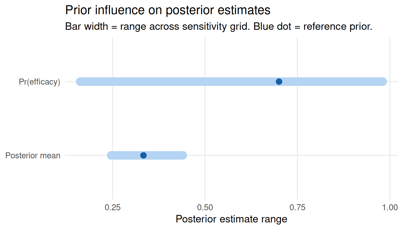

plot_sensitivity(sa, target = "posterior_mean")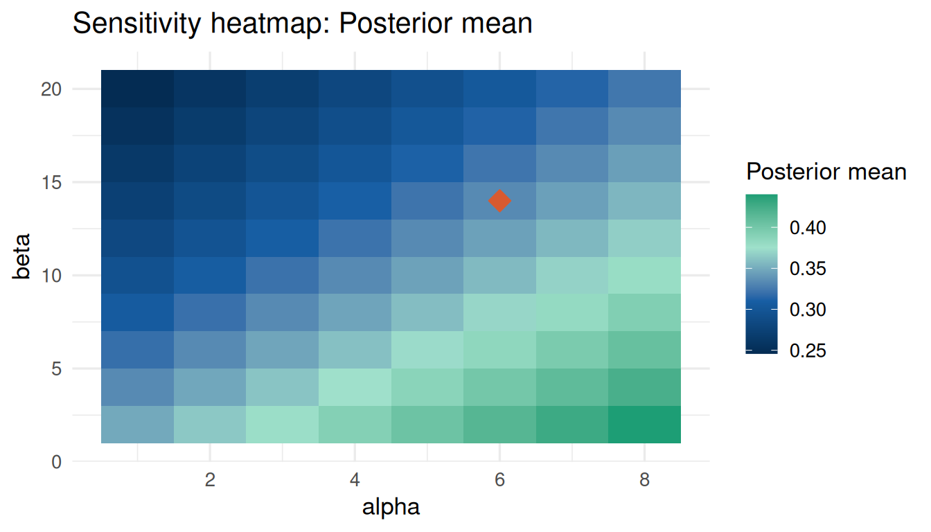

Credible Interval Sensitivity

cri_sa <- sensitivity_cri(
  prior        = prior,
  data_summary = data_obs,
  param_grid   = list(alpha = seq(1, 8, 1), beta = seq(2, 20, 2)),
  cri_level    = 0.95
)
cri_sa$influence_scores

     cri_lower      cri_upper      cri_width posterior_mean   posterior_sd 
    0.15946768     0.21751316     0.06678301     0.19409836     0.01716165

plot_sensitivity(cri_sa, target = "cri_width")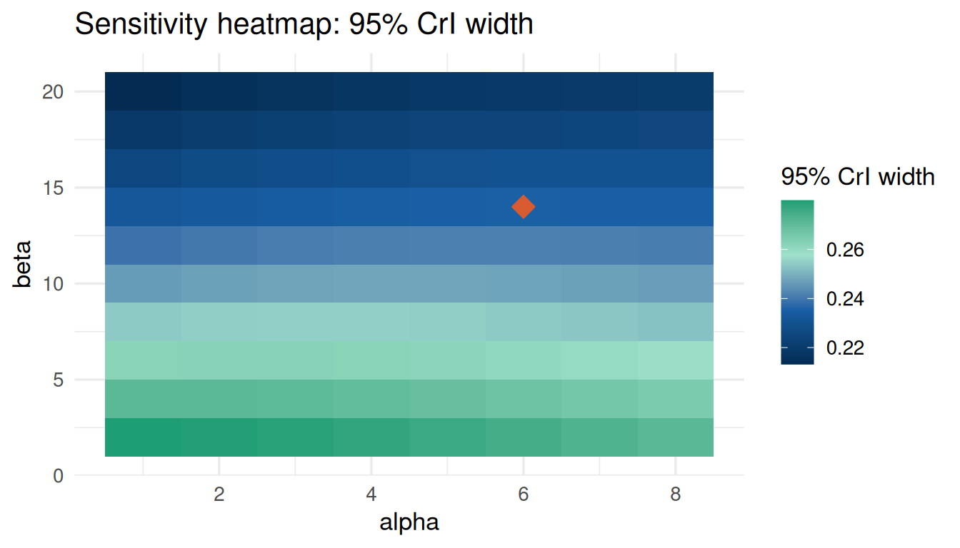

Poisson / Count Data

Sensitivity with Poisson data uses Gamma-Poisson conjugate updating.

prior_ae  <- elicit_gamma(mean = 0.15, sd = 0.06, method = "moments",
                           label = "AE rate (per person-year)")
data_pois <- list(type = "poisson", x = 18, n = 120)

sa_pois <- sensitivity_grid(
  prior        = prior_ae,
  data_summary = data_pois,
  param_grid   = list(shape = seq(2, 10, 1), rate = seq(5, 40, 5)),
  target       = c("posterior_mean", "prob_efficacy"),
  threshold    = 0.20
)
sa_pois$influence_scores

posterior_mean  prob_efficacy 
     0.0990000      0.6908443

plot_tornado(sa_pois)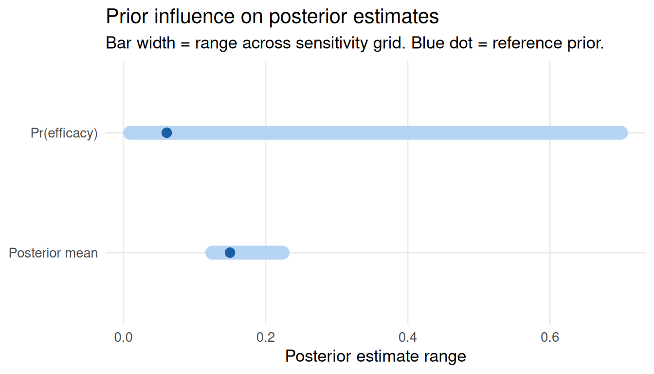

plot_sensitivity(sa_pois, target = "posterior_mean")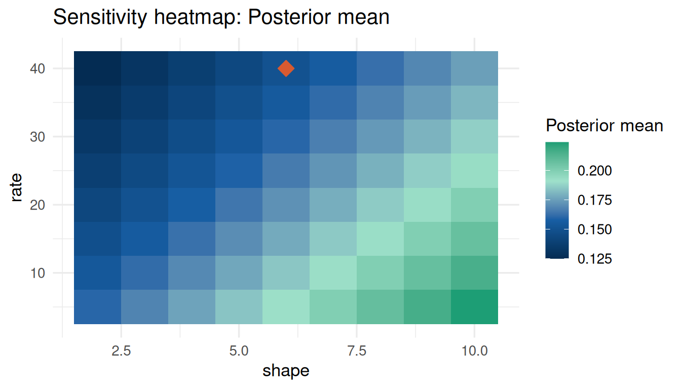

Survival / Time-to-Event Data

Sensitivity with survival data uses Gamma-Exponential conjugate updating.

prior_hz  <- elicit_exponential(mean = 0.05, method = "moments",
                                 label = "OS hazard rate")
data_surv <- list(type = "survival", x = 30, n = 600)

sa_surv <- sensitivity_grid(
  prior        = prior_hz,
  data_summary = data_surv,
  param_grid   = list(shape = seq(1, 5, 0.5), rate = seq(5, 30, 5)),
  target       = c("posterior_mean", "prob_efficacy"),
  threshold    = 0.10
)
sa_surv$influence_scores

posterior_mean  prob_efficacy 
  2.033320e-03   8.021621e-06

plot_tornado(sa_surv)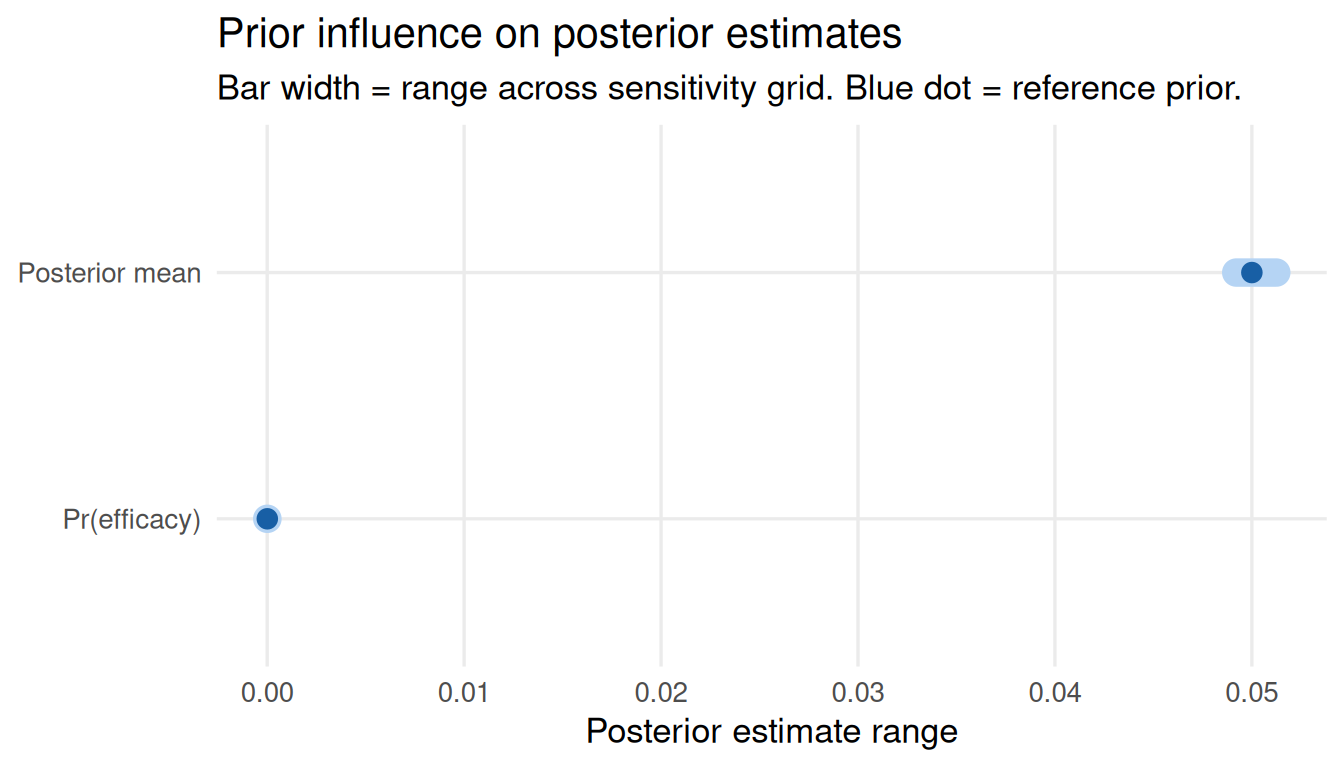

cri_surv <- sensitivity_cri(
  prior        = prior_hz,
  data_summary = data_surv,
  param_grid   = list(shape = seq(1, 5, 0.5), rate = seq(5, 30, 5)),
  cri_level    = 0.95
)
plot_sensitivity(cri_surv, target = "cri_width")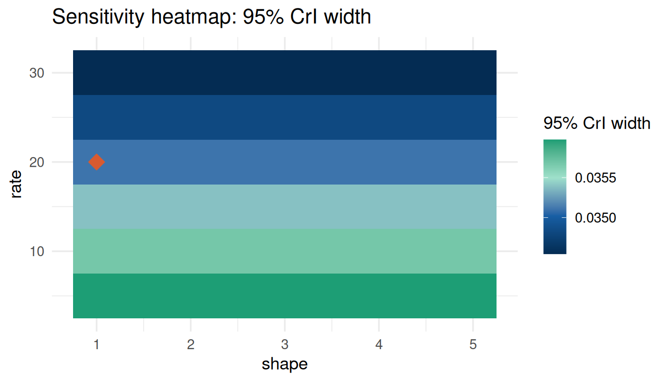

Continuous Endpoints

prior_cont <- elicit_normal(mean = 0.0, sd = 0.3, method = "moments",
                             label = "Log odds ratio")
sa_cont <- sensitivity_grid(
  prior        = prior_cont,
  data_summary = list(type = "continuous", x = 0.20, sd = 0.25, n = 60),
  param_grid   = list(mu = seq(-0.5, 0.5, 0.1), sigma = seq(0.1, 0.8, 0.1)),
  target       = c("posterior_mean", "posterior_sd")
)
plot_tornado(sa_cont)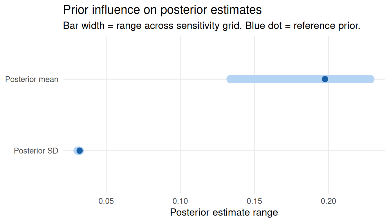

Interpreting Influence Scores

Score	Sensitivity	Implication
< 0.05	Not sensitive	Prior has negligible influence
0.05 – 0.15	Moderate	Report alongside primary estimate
> 0.15	Sensitive	Consider robust prior; emphasise data

Mixture Prior Sensitivity

e1  <- elicit_beta(mean = 0.25, sd = 0.08, method = "moments",
                   expert_id = "E1", label = "ORR")
e2  <- elicit_beta(mean = 0.40, sd = 0.10, method = "moments",
                   expert_id = "E2", label = "ORR")
mix <- aggregate_experts(list(E1 = e1, E2 = e2), weights = c(0.5, 0.5))

sa_mix <- sensitivity_grid(
  prior        = mix,
  data_summary = list(type = "binary", x = 14, n = 40),
  param_grid   = list(alpha = seq(1, 8, 1), beta = seq(2, 16, 2)),
  target       = "posterior_mean"
)
plot_tornado(sa_mix)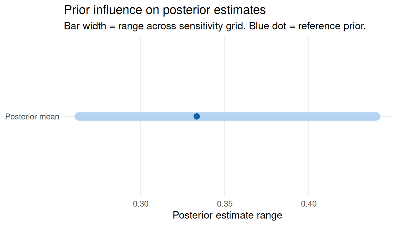

Note: for mixture priors, the grid varies the dominant component’s parameters. A compatibility warning is shown in the Shiny app.

Regulatory Reporting

Include in the clinical study report:

Influence score table — one row per posterior quantity
Tornado plot — ordered from most to least sensitive
Heatmap — for the primary efficacy quantity
Classification statement — sensitive / not sensitive per quantity

All three are generated automatically by prior_report() when a bayprior_sensitivity object is supplied.

References

FDA (2026). Draft Guidance: Bayesian Statistical Methods for Drug and Biological Products.
ICH E9(R1) (2019). Addendum on Estimands and Sensitivity Analysis.