prior <- elicit_beta(
  mean = 0.30, sd = 0.10, method = "moments",
  label = "Response rate"
)Prior-Data Conflict Diagnostics
Why Conflict Diagnostics Matter
Before updating a prior with trial data it is essential to check whether the two are compatible. Substantial prior-data conflict indicates one of three things: the prior was mis-specified, the data are anomalous, or the model is wrong. Regulators increasingly require evidence that conflict was assessed and addressed.
bayprior provides four complementary univariate diagnostics and one multivariate diagnostic, following Box (1980) and related work. The conflict module supports four data types: binary, continuous, Poisson/count, and survival.
Supported Data Types
| Data type | type = argument |
Conjugate update | Typical endpoint |
|---|---|---|---|
| Binary | "binary" |
Beta–Binomial | Response rate, ORR |
| Continuous | "continuous" |
Normal–Normal | Mean difference, HbA1c |
| Poisson / count | "poisson" |
Gamma–Poisson | Adverse event rate |
| Survival | "survival" |
Gamma–Exponential | Hazard rate, OS, PFS |
Univariate Conflict: prior_conflict()
Binary Data
# No-conflict: data consistent with prior
cd_none <- prior_conflict(
  prior        = prior,
  data_summary = list(type = "binary", x = 13, n = 40),
  alpha        = 0.05
)
print(cd_none)
# Mild conflict
cd_mild <- prior_conflict(
prior = prior,
data_summary = list(type = "binary", x = 20, n = 40)
)
print(cd_mild)# Severe conflict
cd_severe <- prior_conflict(
prior = prior,
data_summary = list(type = "binary", x = 35, n = 40)
)
print(cd_severe)The Four Diagnostics Explained
1. Box’s Prior Predictive P-value
\[p_{\text{Box}} = 2\Phi\!\left(-\left|\frac{\hat\theta - \mu_\pi} {\sqrt{\sigma_\pi^2 + \text{SE}^2}}\right|\right)\]
Interpretation: \(p < 0.05\) flags conflict at the 5% level.
2. Surprise Index
\[S = \left|\frac{\hat\theta - \mu_\pi} {\sqrt{\sigma_\pi^2 + \text{SE}^2}}\right|\]
Interpretation: \(S > 2\) moderate; \(S > 3\) high surprise.
3. KL Divergence
\[\text{KL}(P \| Q) = \log\frac{\sigma_Q}{\sigma_P} + \frac{\sigma_P^2 + (\mu_P - \mu_Q)^2}{2\sigma_Q^2} - \frac12\]
Interpretation: \(> 1\) indicates large information distance.
4. Bhattacharyya Overlap Coefficient
\[\text{BC} = \exp\!\left( -\frac{(\mu_P - \mu_Q)^2}{4(\sigma_P^2 + \sigma_Q^2)}\right) \cdot \left(\frac{2\sigma_P\sigma_Q} {\sigma_P^2 + \sigma_Q^2}\right)^{1/2}\]
Interpretation: 1 = identical distributions; 0 = no overlap.
Threshold Summary
| Diagnostic | No conflict | Mild conflict | Severe conflict |
|---|---|---|---|
| Box p-value | >= 0.05 | 0.01-0.05 | < 0.01 |
| Surprise index | < 2 | 2-3 | > 3 |
| KL divergence | < 0.5 | 0.5-1 | > 1 |
| Bhattacharyya overlap | > 0.6 | 0.3-0.6 | < 0.3 |
Prior-Likelihood-Posterior Overlay
plot_prior_likelihood(
  prior,
  data_summary   = list(type = "binary", x = 13, n = 40),
  show_posterior = TRUE
)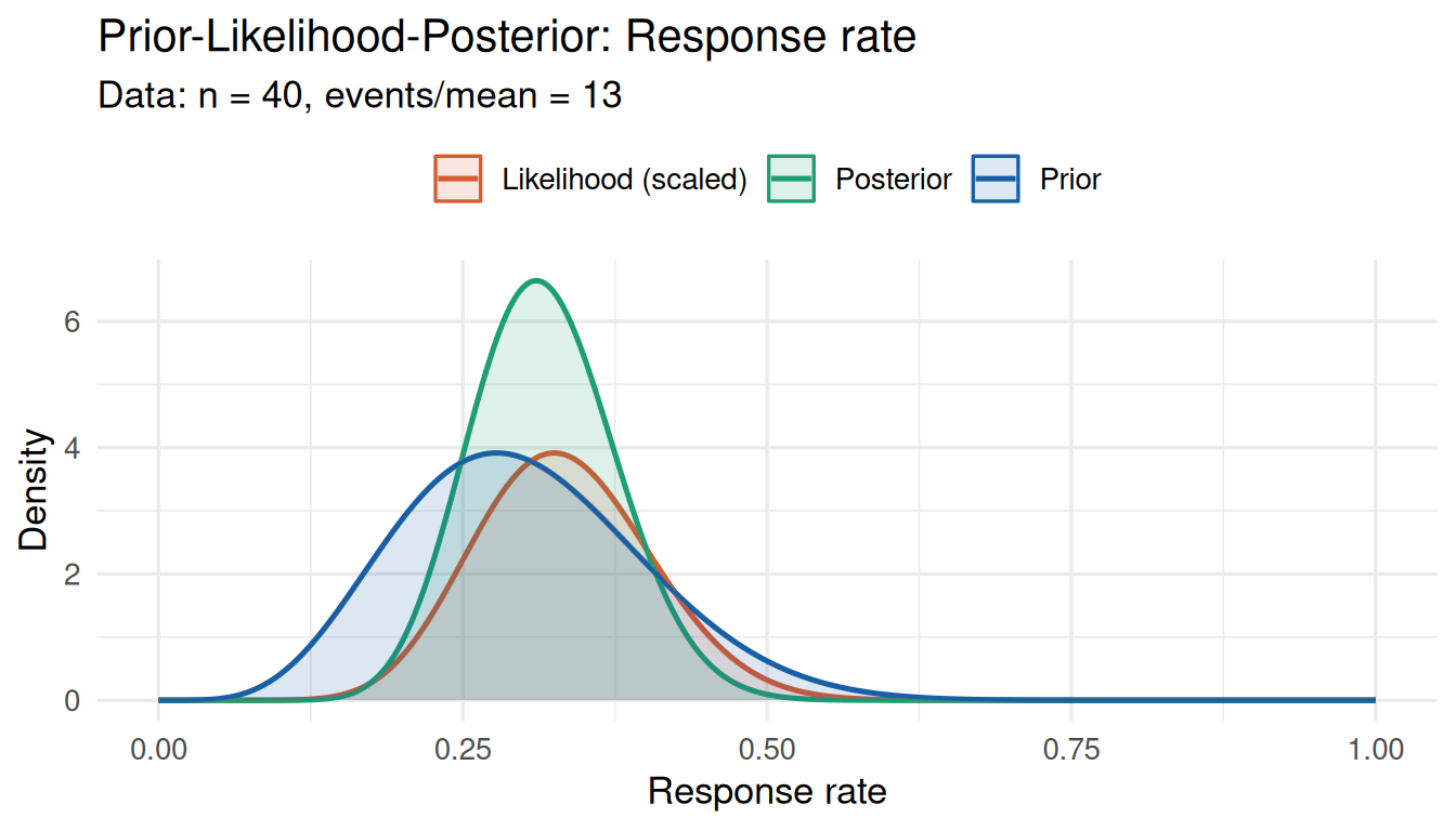
No conflict: prior and likelihood overlap substantially.
plot_prior_likelihood(
  prior,
  data_summary   = list(type = "binary", x = 35, n = 40),
  show_posterior = TRUE
)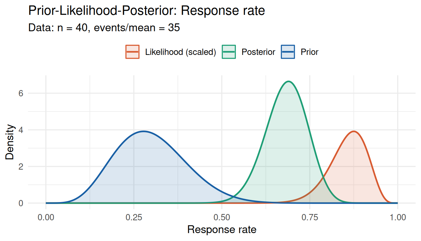
Severe conflict: prior (blue) and likelihood (orange) widely separated.
Continuous Endpoint Conflict
prior_norm <- elicit_normal(
  mean = 0.0, sd = 0.3, method = "moments",
  label = "Log odds ratio"
)

# No conflict: observed log OR consistent with prior
prior_conflict(
  prior_norm,
  data_summary = list(type = "continuous", x = 0.15, sd = 0.20, n = 80)
)
Poisson / Count Data Conflict
Poisson/count data arises for endpoints such as adverse event rates, where the observed data consists of a count of events over an exposure period (person-time). The conjugate update uses a Gamma-Poisson model:
\[\text{Prior: Gamma}(\alpha, \beta) \quad\Rightarrow\quad \text{Posterior: Gamma}(\alpha + x,\; \beta + n)\]
where \(x\) = observed events and \(n\) = total person-time.
# Gamma prior on adverse event rate
# Expert believes the AE rate is ~0.15 events per person-year (SD 0.06)
prior_ae <- elicit_gamma(
  mean      = 0.15,
  sd        = 0.06,
  method    = "moments",
  label     = "Adverse event rate (per person-year)",
  expert_id = "Safety Expert"
)
print(prior_ae)
# Observed: 12 AEs over 100 person-years => rate 0.12 — consistent with prior
cd_pois_none <- prior_conflict(
prior = prior_ae,
data_summary = list(type = "poisson", x = 12, n = 100),
alpha = 0.05
)
print(cd_pois_none)# Observed: 40 AEs over 100 person-years => rate 0.40 — much higher than prior
cd_pois_conf <- prior_conflict(
prior = prior_ae,
data_summary = list(type = "poisson", x = 40, n = 100)
)
print(cd_pois_conf)plot_prior_likelihood(
prior_ae,
data_summary = list(type = "poisson", x = 40, n = 100),
show_posterior = TRUE
)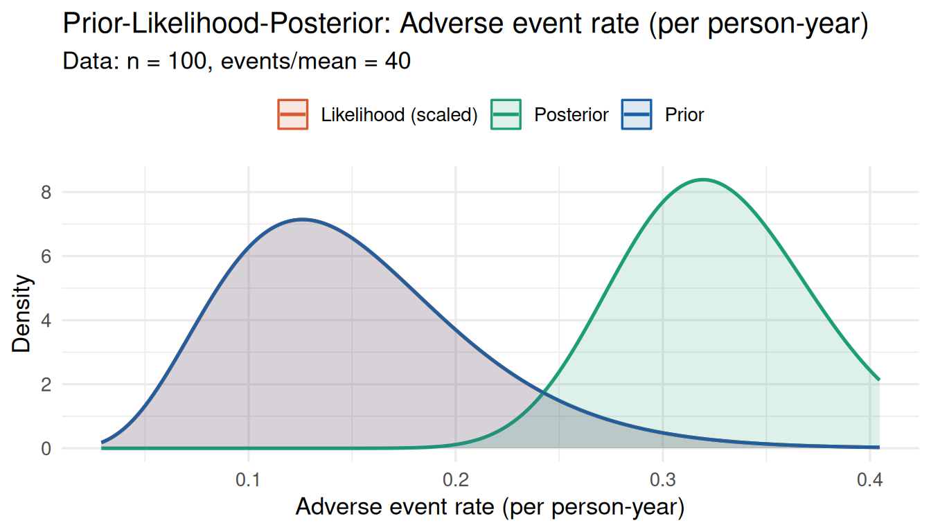
Survival / Time-to-Event Data Conflict
Survival data conflict arises for endpoints like OS and PFS hazard rates. The observed data consists of event counts over a total follow-up time (person-months). The conjugate update uses a Gamma-Exponential model:
\[\text{Prior: Gamma}(\alpha, \beta) \quad\Rightarrow\quad \text{Posterior: Gamma}(\alpha + d,\; \beta + T)\]
where \(d\) = observed events and \(T\) = total follow-up time.
An Exponential prior (constant hazard) is equivalent to \(\text{Gamma}(1, \lambda)\).
# Exponential prior on hazard rate
# Expert believes median OS ≈ 20 months => hazard ≈ 0.05
prior_hz <- elicit_exponential(
  mean      = 0.05,
  method    = "moments",
  label     = "OS hazard rate",
  expert_id = "Clinical Expert"
)
print(prior_hz)
# Observed: 20 deaths over 400 person-months => hazard 0.05 — consistent
cd_surv_none <- prior_conflict(
prior = prior_hz,
data_summary = list(type = "survival", x = 20, n = 400),
alpha = 0.05
)
print(cd_surv_none)# Observed: 60 deaths over 400 person-months => hazard 0.15 — much higher
cd_surv_conf <- prior_conflict(
prior = prior_hz,
data_summary = list(type = "survival", x = 60, n = 400)
)
print(cd_surv_conf)plot_prior_likelihood(
prior_hz,
data_summary = list(type = "survival", x = 60, n = 400),
show_posterior = TRUE
)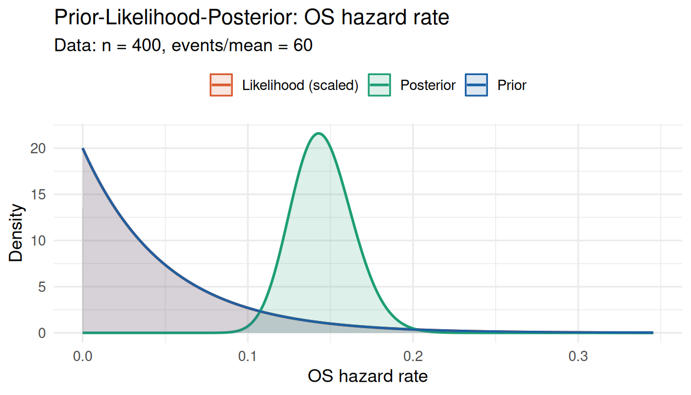
Also works with a Gamma prior on the hazard rate:
prior_hz_gamma <- elicit_gamma(
  mean = 0.05, sd = 0.02, method = "moments",
  label = "OS hazard rate (Gamma prior)"
)
prior_conflict(
  prior_hz_gamma,
  data_summary = list(type = "survival", x = 20, n = 400)
)
Compatibility Validation
bayprior warns when the prior family is atypical for the chosen data type, helping users avoid inadvertent misspecification:
# Warning: Beta prior with Poisson data is unusual
prior_beta <- elicit_beta(mean = 0.15, sd = 0.06, method = "moments",
                           label = "Rate")
# The app shows a warning notification; the function still runs with
# a Normal approximation
cd_warn <- prior_conflict(
  prior_beta,
  data_summary = list(type = "poisson", x = 15, n = 100)
)
Mixture Prior Conflict
All diagnostics work transparently with mixture priors via a Normal approximation from the mixture’s fit_summary:
e1 <- elicit_beta(mean = 0.25, sd = 0.08, method = "moments",
                  expert_id = "E1", label = "ORR")
e2 <- elicit_beta(mean = 0.40, sd = 0.12, method = "moments",
                  expert_id = "E2", label = "ORR")
mix <- aggregate_experts(list(E1 = e1, E2 = e2), weights = c(0.5, 0.5))

prior_conflict(mix, list(type = "binary", x = 18, n = 40))
Multivariate Conflict: conflict_mahalanobis()
For trials with co-primary endpoints, the Mahalanobis distance provides an omnibus multivariate conflict test:
conflict_mahalanobis(
  prior_means = c(0.35, 0.60),
  prior_cov   = matrix(c(0.010, 0.003, 0.003, 0.015), 2, 2),
  obs_means   = c(0.55, 0.58),
  obs_cov     = matrix(c(0.008, 0.002, 0.002, 0.010), 2, 2) / 50,
  labels      = c("Response rate", "OS rate"),
  alpha       = 0.05
)
Marginal z-scores per parameter:
Response rate       OS rate
        1.984        -0.162
Conflict Severity Classification
| Severity | Recommended action |
|---|---|
| None | Proceed — prior is consistent with data |
| Mild | Consider reporting both prior-weighted and likelihood-only estimates |
| Severe | Revise prior or use a robust/power prior; report sensitivity |
References
- Box, G. E. P. (1980). Sampling and Bayes’ inference in scientific modelling and robustness. JRSS-A, 143, 383–430.
- Bhattacharyya, A. (1943). On a measure of divergence between two statistical populations. Bulletin of the Calcutta Mathematical Society, 35, 99–109.