Prior Elicitation Methods

Author

Ndoh Penn

Published

May 17, 2026

Overview

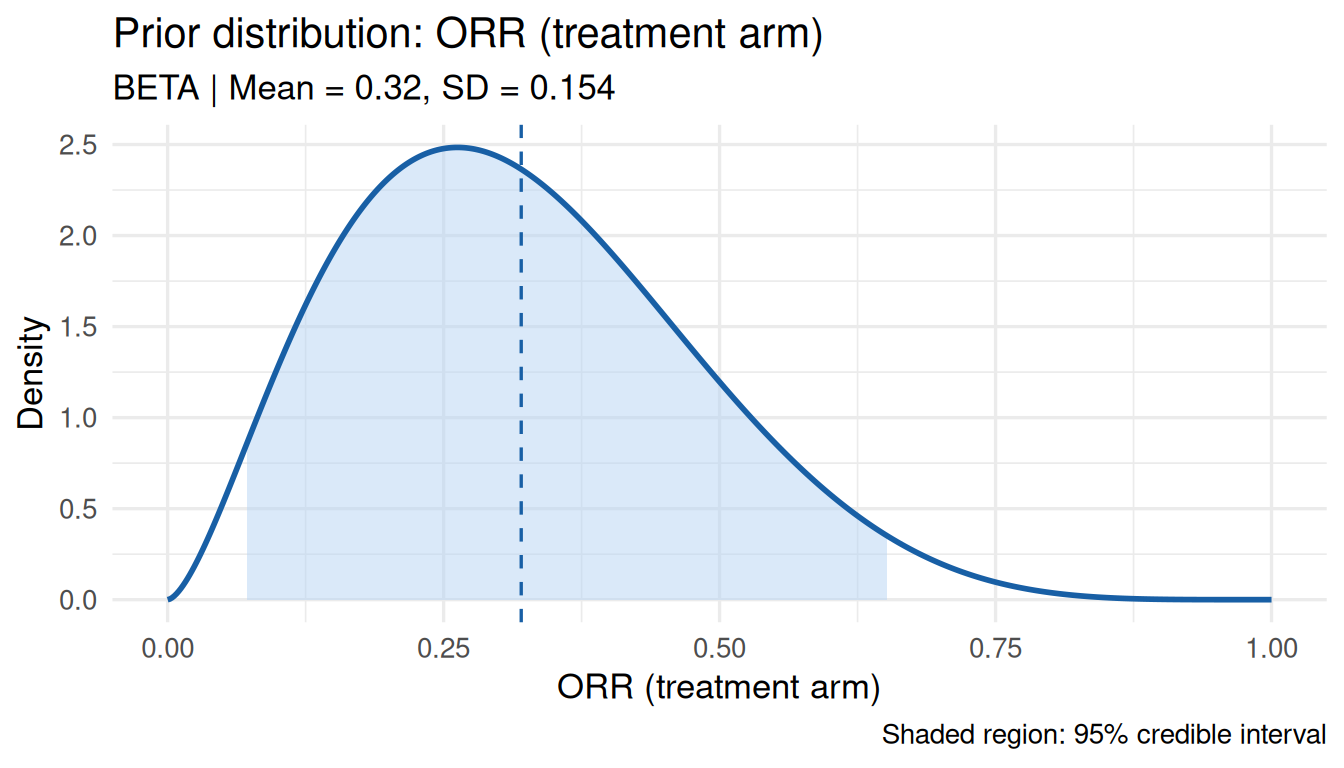
Prior elicitation translates an expert’s subjective beliefs about an unknown quantity into a formal probability distribution. bayprior implements the SHELF methodology (O’Hagan et al., 2006) across six distribution families and three elicitation methods.

Distribution Families

Family	Support	Typical quantity
Beta	(0, 1)	Response rates, proportions
Normal	(−∞, ∞)	Mean differences, log odds ratios
Gamma	(0, ∞)	Event rates, median survival
Log-Normal	(0, ∞)	Hazard ratios, PK parameters
Exponential	(0, ∞)	Constant hazard rates, Poisson rate priors
Weibull	(0, ∞)	Non-constant hazard survival times (OS, PFS)

Elicitation Methods

Quantile matching — expert specifies probability–value pairs
Moment matching — expert specifies mean and SD
Roulette — expert allocates chips across histogram bins

Beta Prior (Binary Endpoints)

Quantile Matching

prior_q <- elicit_beta(
  quantiles = c("0.05" = 0.10, "0.50" = 0.30, "0.95" = 0.60),
  expert_id = "Expert_1",
  label     = "ORR (treatment arm)"
)
print(prior_q)
plot(prior_q)

Moment Matching

prior_m <- elicit_beta(
  mean      = 0.30,
  sd        = 0.10,
  method    = "moments",
  expert_id = "Expert_1",
  label     = "ORR (treatment arm)"
)
print(prior_m)

Moment matching solves analytically: \[\alpha = \mu \left(\frac{\mu(1-\mu)}{\sigma^2} - 1\right), \quad \beta = (1-\mu)\left(\frac{\mu(1-\mu)}{\sigma^2} - 1\right)\]

Normal Prior (Continuous Endpoints)

prior_lor <- elicit_normal(
  quantiles = c("0.025" = -0.50, "0.50" = 0.20, "0.975" = 0.90),
  label     = "Log odds ratio"
)
plot(prior_lor)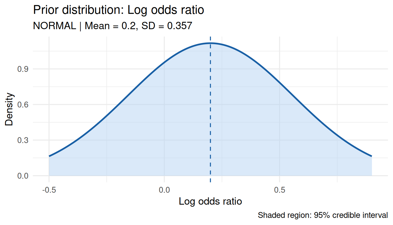

prior_md <- elicit_normal(
  mean = 0.0, sd = 0.5, method = "moments",
  label = "Mean difference (sceptical)"
)
plot(prior_md)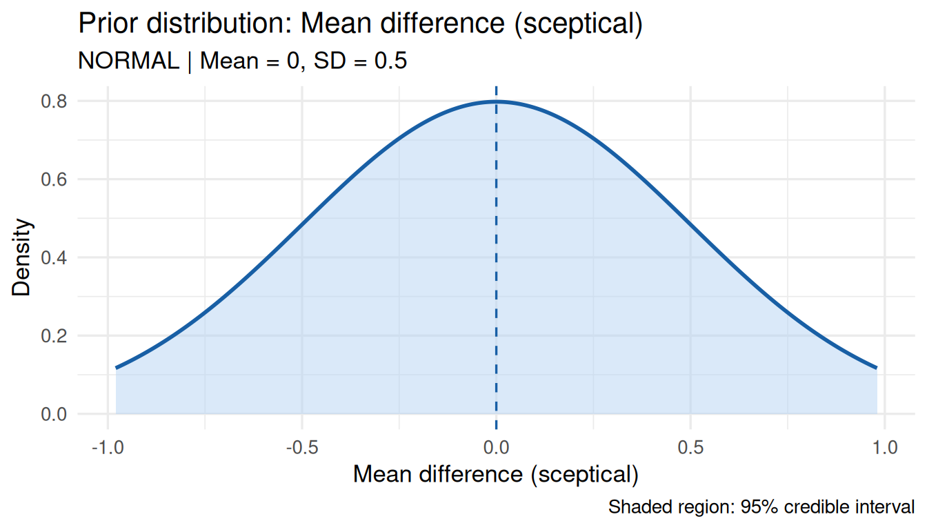

Gamma Prior (Rate and Count Endpoints)

The Gamma distribution is the conjugate prior for Poisson and exponential likelihoods — a natural choice for event rate priors.

prior_os <- elicit_gamma(
  mean = 18, sd = 6, method = "moments",
  label = "Median OS (months)"
)
plot(prior_os)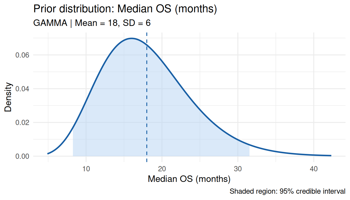

prior_rate <- elicit_gamma(
  quantiles = c("0.10" = 2, "0.50" = 5, "0.90" = 10),
  label     = "Event rate (per 100 patient-years)"
)
print(prior_rate)

\[\text{mean} = \frac{\text{shape}}{\text{rate}}, \quad \text{SD} = \frac{\sqrt{\text{shape}}}{\text{rate}}\]

Log-Normal Prior (Hazard Ratios)

prior_hr <- elicit_lognormal(
  quantiles = c("0.05" = 0.40, "0.50" = 0.70, "0.95" = 1.20),
  label     = "Hazard ratio (treatment vs control)"
)
plot(prior_hr)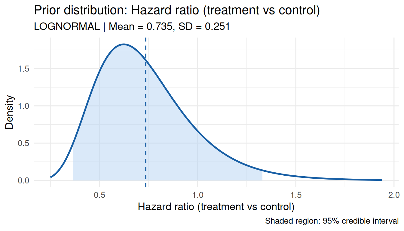

prior_pk <- elicit_lognormal(
  mean = 25, sd = 10, method = "moments",
  label = "AUC (ng/mL*h)"
)
print(prior_pk)

Exponential Prior (Constant Hazard Rates)

The Exponential distribution models a constant hazard rate $\lambda > 0$. The mean is $1/\lambda$ and the SD equals the mean. It is the conjugate prior likelihood for Gamma priors on Poisson rates, and is appropriate when the hazard rate is assumed constant over time.

Use cases: adverse event rates (events per person-time), constant-hazard survival endpoints, Poisson rate priors for count data.

Method: moments

# Mean hazard rate 0.05 => mean survival 1/0.05 = 20 months
prior_hz <- elicit_exponential(
  mean      = 0.05,
  method    = "moments",
  label     = "Hazard rate (constant)",
  expert_id = "Expert_1"
)
print(prior_hz)
plot(prior_hz)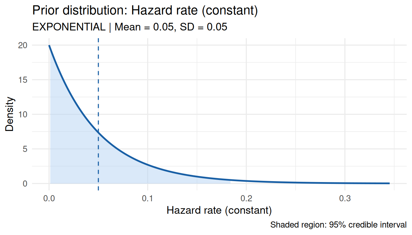

Method: rate

Direct rate specification (= $\lambda$):

prior_ae <- elicit_exponential(
  rate   = 0.12,
  method = "rate",
  label  = "AE rate per person-year"
)
print(prior_ae)

Method: quantile

Fit the rate from expert-specified quantiles:

prior_hz_q <- elicit_exponential(
  quantiles = c("0.25" = 0.02, "0.50" = 0.05, "0.75" = 0.10),
  method    = "quantile",
  label     = "Hazard rate"
)
print(prior_hz_q)
plot(prior_hz_q)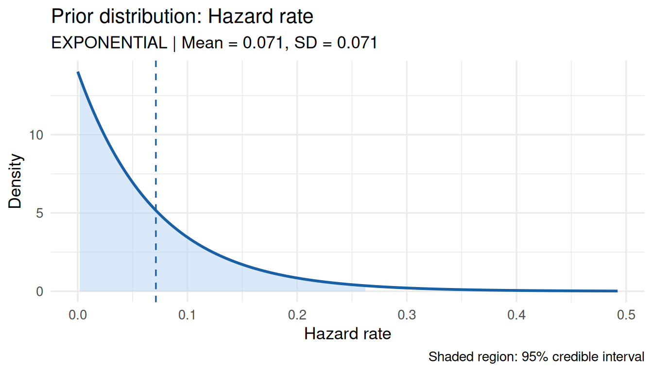

Conjugate update

With Poisson/survival data:

\[\text{Prior: Exponential}(\lambda) \approx \text{Gamma}(1, \lambda)\] \[\text{Posterior: Gamma}(1 + x,\; \lambda + n)\]

where $x$ = observed events, $n$ = exposure time or follow-up.

Weibull Prior (Non-Constant Hazard Survival Times)

The Weibull distribution is the most widely used model for survival analysis. It is parameterised by shape $k > 0$ and scale $\lambda > 0$:

\[\text{mean} = \lambda\,\Gamma(1 + 1/k), \quad \text{SD} = \lambda\sqrt{\Gamma(1 + 2/k) - \Gamma(1 + 1/k)^2}\]

Shape parameter interpretation:

Shape $k$	Hazard	Clinical scenario
$k < 1$	Decreasing	Early frailty, selection
$k = 1$	Constant	Equivalent to Exponential
$k > 1$	Increasing	Ageing, post-surgical deterioration

Method: moments

Specify prior mean and SD — bayprior solves for shape and scale via Nelder-Mead optimisation:

prior_wb <- elicit_weibull(
  mean      = 20,
  sd        = 10,
  method    = "moments",
  label     = "OS (months)",
  expert_id = "Expert_1"
)
print(prior_wb)
plot(prior_wb)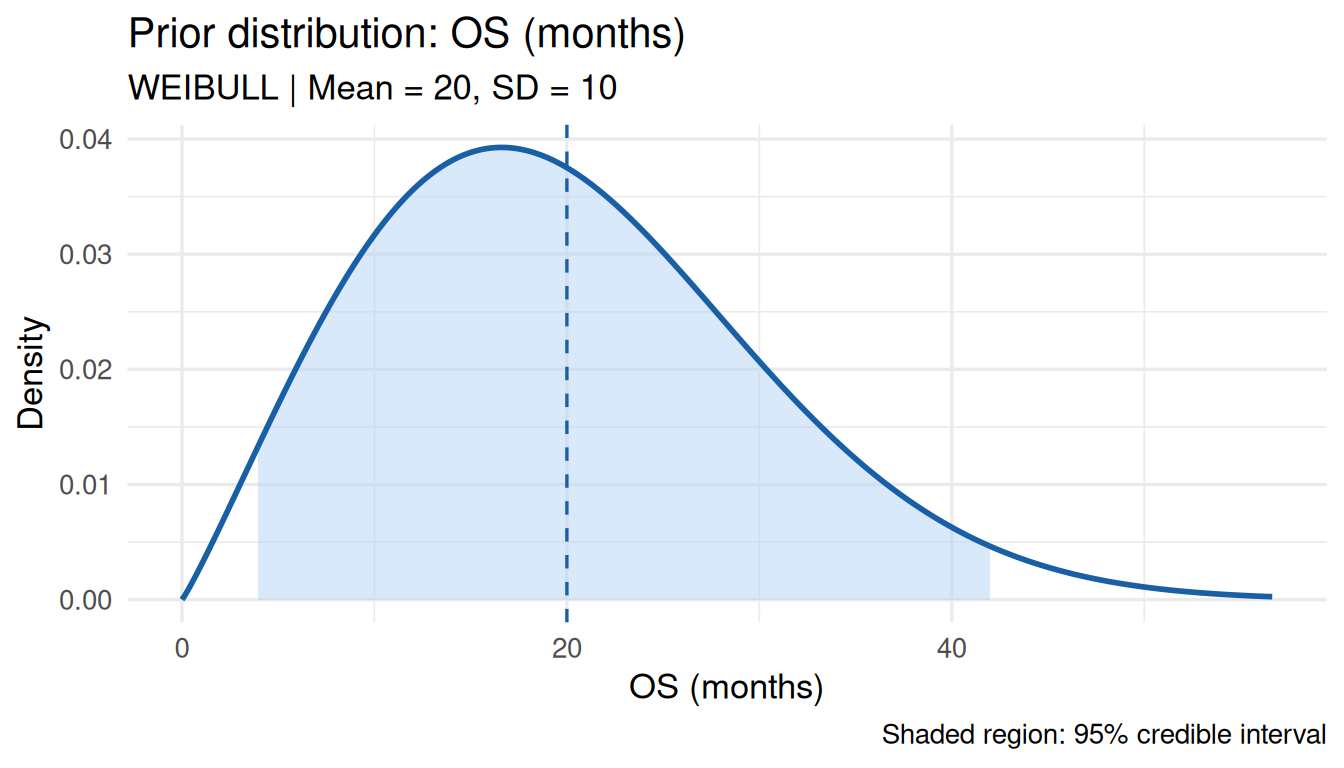

Method: params

Direct shape and scale specification:

# k=2: linearly increasing hazard
prior_wb2 <- elicit_weibull(
  shape  = 2,
  scale  = 20,
  method = "params",
  label  = "PFS (months) — increasing hazard"
)
print(prior_wb2)
plot(prior_wb2)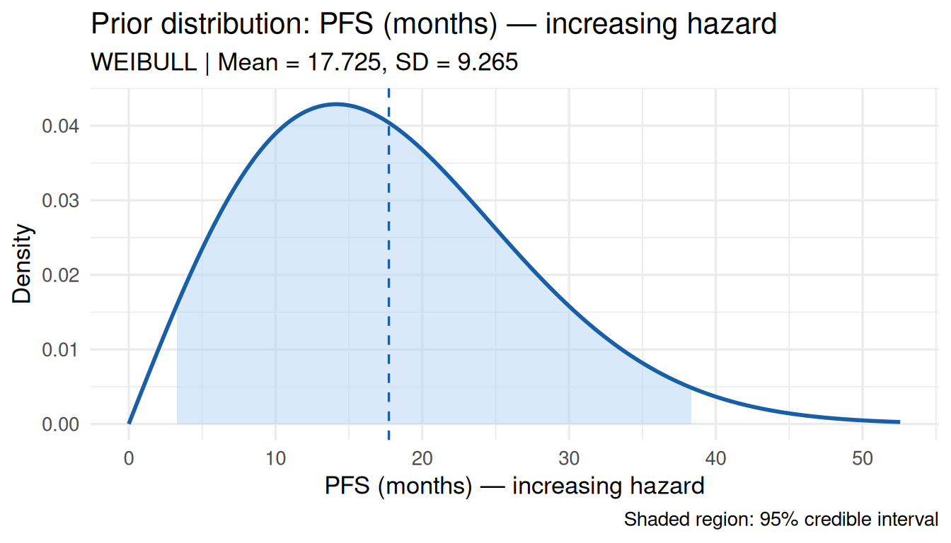

Method: quantile

prior_wb3 <- elicit_weibull(
  quantiles = c("0.10" = 5, "0.50" = 18, "0.90" = 40),
  method    = "quantile",
  label     = "OS (months)"
)
print(prior_wb3)
plot(prior_wb3)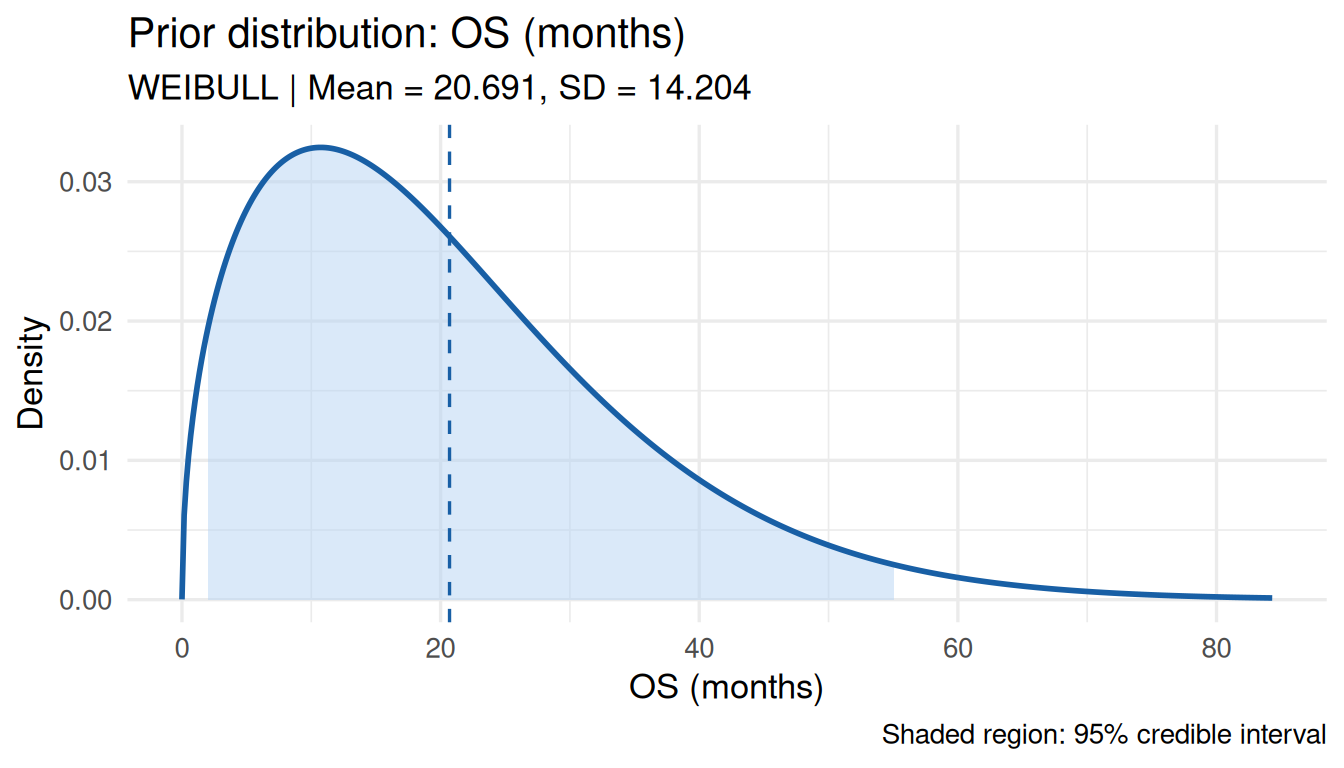

Posterior approximation note

The Weibull distribution does not have a closed-form conjugate prior. When used in prior_conflict() or sensitivity_grid(), bayprior applies a Normal approximation to the posterior matched to the Weibull’s fit_summary moments.

Roulette Method

The interactive chip-allocation method for clinical experts unfamiliar with probability distributions. In the Shiny app this is fully interactive; programmatically:

prior_rou <- elicit_roulette(
  chips  = c(0L, 1L, 3L, 7L, 9L, 7L, 4L, 2L, 1L, 1L),
  breaks = seq(0, 1, by = 0.1),
  family = "beta",
  label  = "Response rate"
)
print(prior_rou)
plot(prior_rou)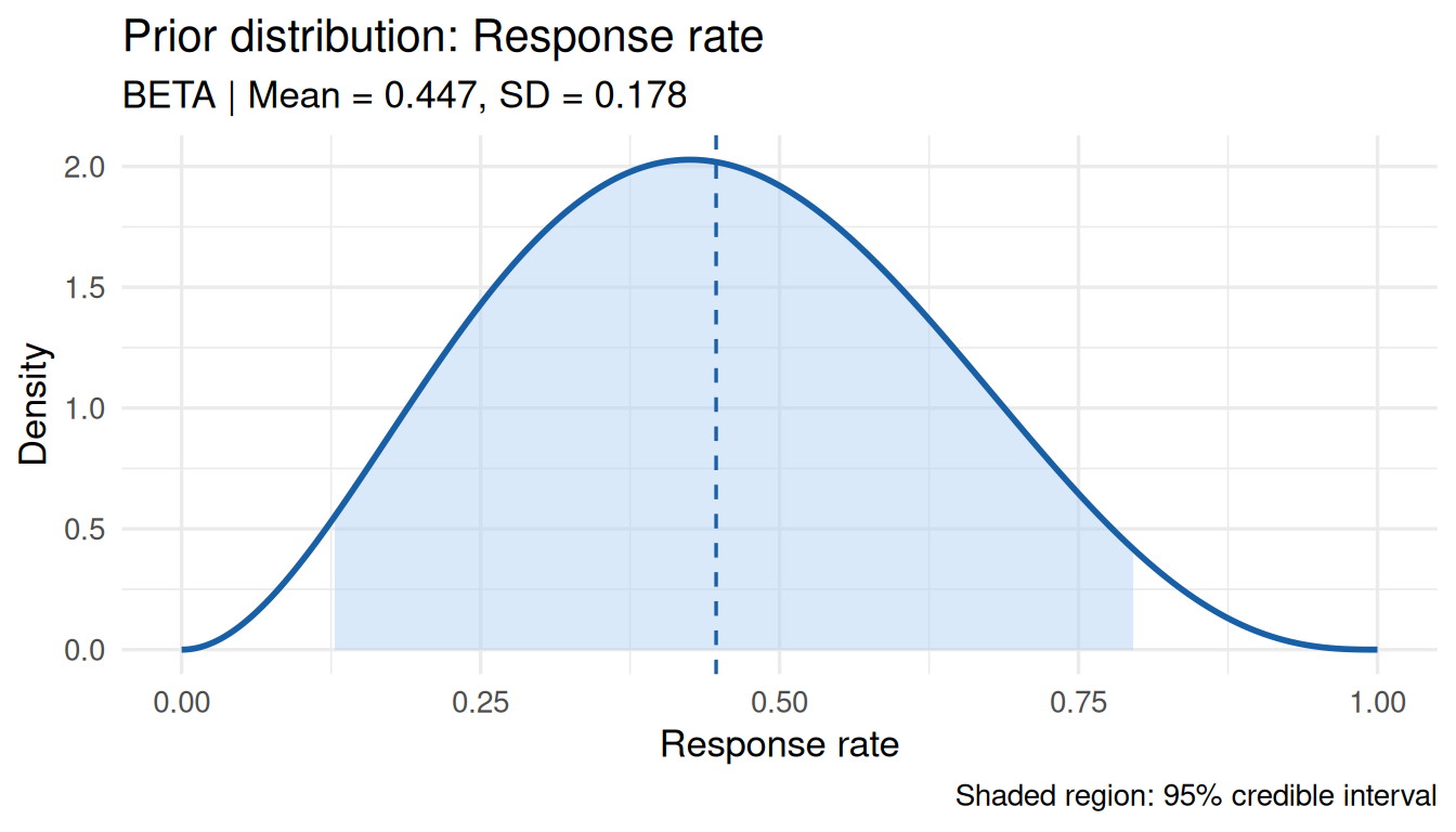

Expert Pooling

Linear Pooling

e1 <- elicit_beta(mean = 0.25, sd = 0.08, method = "moments",
                  expert_id = "Oncologist_1", label = "ORR")
e2 <- elicit_beta(mean = 0.35, sd = 0.10, method = "moments",
                  expert_id = "Oncologist_2", label = "ORR")
e3 <- elicit_beta(
  quantiles = c("0.10" = 0.15, "0.50" = 0.30, "0.90" = 0.52),
  expert_id = "Statistician", label = "ORR"
)
consensus <- aggregate_experts(
  priors  = list(Oncologist_1 = e1, Oncologist_2 = e2, Statistician = e3),
  weights = c(0.40, 0.35, 0.25),
  method  = "linear"
)
plot(consensus)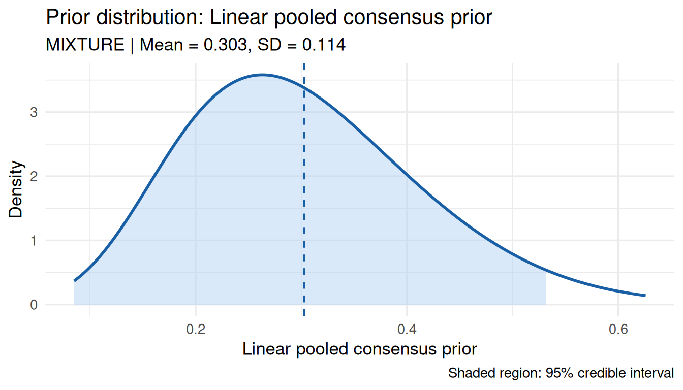

Pooling Compatibility

bayprior validates compatibility before pooling. Priors with incompatible supports (e.g. Beta + Normal) are blocked with an error. Same-support cross-family pooling (e.g. Gamma + Exponential) proceeds with a warning noting that sensitivity analysis will use the dominant component’s parameters.

# Same positive support — allowed (Gamma + Exponential)
g1   <- elicit_gamma(mean = 5, sd = 2, method = "moments",
                     expert_id = "E1", label = "Rate")
exp1 <- elicit_exponential(mean = 0.2, method = "moments",
                            expert_id = "E2", label = "Rate")
pool_pos <- aggregate_experts(
  priors  = list(E1 = g1, E2 = exp1),
  weights = c(0.5, 0.5)
)
print(pool_pos)

Prior Object Structure

All elicit_*() functions return a "bayprior" S3 object:

str(prior_q, max.level = 1)

List of 7
 $ dist       : chr "beta"
 $ params     :List of 2
 $ method     : chr "quantile"
 $ expert_id  : chr "Expert_1"
 $ label      : chr "ORR (treatment arm)"
 $ input      :List of 1
 $ fit_summary:List of 5
 - attr(*, "class")= chr "bayprior"

Slot	Content
`$dist`	Family: `"beta"`, `"normal"`, `"gamma"`, `"lognormal"`, `"exponential"`, `"weibull"`, `"mixture"`
`$params`	Named list of fitted hyperparameters
`$fit_summary`	`mean`, `sd`, `q025`, `q500`, `q975`
`$method`	Elicitation method
`$expert_id`	Expert identifier
`$label`	Quantity label

References

O’Hagan, A. et al. (2006). Uncertain Judgements: Eliciting Experts’ Probabilities. Wiley.
Oakley, J. E. & O’Hagan, A. (2010). SHELF: the Sheffield Elicitation Framework. University of Sheffield.